National Radio
Astronomy Observatory

5.2.5.1 Mode mfs

The default mode=’mfs’ emulates multi-frequency synthesis in that each visibility-channel datum k with baseline vector B_k at wavelength λ_k is gridded into the uv-plane at u_k = B_k∕λ_k. The result is one or more images (depending on nterms), regardless of how many channels are in the input dataset. The first image plane is at the frequency given by the midpoint between the highest and lowest frequency channels in the input spw(s). Currently, there is no way to choose the center frequency of the output image plane independently.

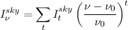
WideBand imaging (mfs with nterms> 1) is now available in CASA. This algorithm models the wide-band sky brightness as a linear combination of Gaussian-like functions whose amplitudes follow a Taylor-polynomial in frequency. The output images are a set of Taylor-coefficient images, from which spectral index and curvature maps are derived. The reffreq parameter sets the reference frequency ν₀ about which the Taylor expansion is done. The Taylor expansion is a polynomial in frequency:

(5.1)

I_t^sky an image of the t^th coefficient of the Taylor-polynomial expansion.

When Eq. 5.1 is applied on a source with a spectral index

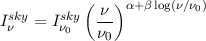(5.2)

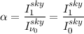
The Taylor terms I_t^sky can be used to constrain the sky brightness, α, and β through

(5.3)

(5.4)

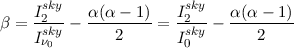(5.5)

For more information, please see Rau, U. & Cornwell, T. J. 2011, “A multi-scale multi-frequency deconvolution algorithm for synthesis imaging in radio interferometry”, A&A, 532, 71

Alert: The MS-MFS (multiscale-multifrequency) algorithm in the current release is new and is still being developed/tested/debugged. Its basic operation has been tested on wide-band JVLA data for Stokes I imaging.

Explanation of the Parameters:
nterms: The number of terms in the Taylor polynomial used to model the frequency structure. nterms> 1 triggers MS-MFS. nterms= 1 triggers standard point-source clean or multi-scale-clean. Note: The choice of nterms follows the same rules used while fitting a polynomial to a 1D set of noisy data points. To prevent overfitting, the order of the polynomial needs to depend on the available signal-to-noise in the data. A very rough rule-of-thumb is as follows: For high SNR data (single channel SNR>100), and fields dominated by point-sources with spectral indices around -1.0 across a 2:1 bandwidth, choose nterms= 3 or 4. For lower SNR data (5 <SNR< 100), flatter spectra, or when there is significant extended emission, nterms= 2 is a much safer option. For very low SNR data (SNR< 5), choose nterms= 1).

reffreq: The reference frequency used to compute Taylor functions [(freq -reffreq)∕(reffreq)]ⁱ. If left blank (reffreq=”), it defaults to the middle frequency of the selected data. Note : For the current release, the use of reffreq=” is recommended.

multiscale: The MS-MFS algorithm always uses scale sizes set via the multiscale parameter. For point-source deconvolution, set multiscale=[0] (also the default). Note: Unlike standard msclean (multiscale = [0,6,10,....] with nterms=1), with higher nterms the largest specified scale size must lie within the sampled range of the interferometer. If not, there can be an ambiguity in the spectral reconstruction at very large spatial scales.

gridmode: Wideband W-Projection is supported, and can be triggered via gridmode=’widefield’.

modelimage: Supply a list of Taylor-coefficient images, to start the deconvolution from. If only one image is specified, it will be used as the model for the ’tt0’ image.

Output images: [xxx.image.tt0, xxx.image.tt1,... ] : Images of Taylor coefficients that describe the frequency-structure. The ”tt0” image is the total-intensity image at the reference frequency, and is equivalent to ”xxx.image” obtained via standard imaging.

[xxx.image.alpha, xxx.image.beta] : Spectral index and spectral curvature at the reference-frequency. These are computed from tt0, tt1, tt2 only for regions of the image where there is sufficient signal-to-noise to compute them. These regions are chosen via a threshold on the intensity image (tt0) computed as MAX( userthreshold*5 , peakresidual/10 ) ). This threshold is reported in the logger. Elsewhere, the values are currently set to zero.

[xxx.image.alpha.error] contains the errors of the spectral index solutions.

The following is a list of differences between MS-MFS (nterms> 1) and standard imaging, in the current CASA release.

1. Iterations always proceed as cs-clean major/minor cycles, and uses the full psf during minor cycle iterations. There are currently no user-controls on the cyclespeedup, and the flux-limit per major cycle is chosen as 10% of the peak residual. In future releases, this will be made more adaptive/controllable.
2. Currently, the following options are not supported for nterms> 1: psfmode, pbcorr, minpb, imagermode=’mosaic’, gridmode=’aprojection’, cyclespeedup, and allowed are one of Stokes I, Q, U, V, RR, LL, XX, YY at a time. More options and combinations are currently under development and testing. Under ’Using CASA’ → ’Other Documentation’ → ’Imaging Algorithms in CASA’ you can find the latest implementations.

More information about CASA may be found at the CASA web page

Copyright © 2010 Associated Universities Inc., Washington, D.C.

This code is available under the terms of the GNU General Public Lincense