Single Dish Spectral Analysis Use Case With ASAP Toolkit

NRAO Home > CASA > CASA Cookbook and User Reference Manual

8.3.11 Single Dish Spectral Analysis Use Case With ASAP Toolkit

Below is a script that illustrates how to reduce single dish data using ASAP within CASA. First a summary of the dataset is given and then the script.

#           MeasurementSet Name:  /home/rohir3/jocular/SD/OrionS_rawACSmod      MS Version 2
#
# Project: AGBT06A_018_01
# Observation: GBT(1 antennas)
#
#Data records: 256       Total integration time = 1523.13 seconds
#   Observed from   01:45:58   to   02:11:21
#
#Fields: 4
#  ID   Name          Right Ascension  Declination   Epoch
#  0    OrionS        05:15:13.45      -05.24.08.20  J2000
#  1    OrionS        05:35:13.45      -05.24.08.20  J2000
#  2    OrionS        05:15:13.45      -05.24.08.20  J2000
#  3    OrionS        05:35:13.45      -05.24.08.20  J2000
#
#Spectral Windows:  (8 unique spectral windows and 1 unique polarization setups)
#  SpwID  #Chans Frame Ch1(MHz)    Resoln(kHz) TotBW(kHz)  Ref(MHz)    Corrs
#  0        8192 LSRK  45464.3506  6.10423298  50005.8766  45489.3536  RR  LL HC3N
#  1        8192 LSRK  45275.7825  6.10423298  50005.8766  45300.7854  RR  LL HN15CO
#  2        8192 LSRK  44049.9264  6.10423298  50005.8766  44074.9293  RR  LL CH3OH
#  3        8192 LSRK  44141.2121  6.10423298  50005.8766  44166.2151  RR  LL HCCC15N
#  12       8192 LSRK  43937.1232  6.10423356  50005.8813  43962.1261  RR  LL HNCO
#  13       8192 LSRK  42620.4173  6.10423356  50005.8813  42645.4203  RR  LL H15NCO
#  14       8192 LSRK  41569.9768  6.10423356  50005.8813  41594.9797  RR  LL HNC18O
#  15       8192 LSRK  43397.8198  6.10423356  50005.8813  43422.8227  RR  LL SiO

# Scans: 21-24  Setup 1 HC3N et al
# Scans: 25-28  Setup 2 SiO et al

casapath=os.environ[’AIPSPATH’]

#ASAP script                            # COMMENTS
#-------------------------------------- -----------------------------------------------
import asap as sd                       #import ASAP package into CASA
                                        #Orion-S (SiO line reduction only)
                                        #Notes:
                                        #scan numbers (zero-based) as compared to GBTIDL

                                        #changes made to get to OrionS_rawACSmod
                                        #modifications to label sig/ref positions
os.environ[’AIPSPATH’]=casapath         #set this environment variable back - ASAP changes it

s=sd.scantable(’OrionS_rawACSmod’,False)#load the data without averaging

Figure 8.6: Multi-panel display of the scantable. Subpanels are displayed per scan. There are two spectra in each scan indicating two polarization (RR and LL).

_________________________________________________________________________________________

s.summary()                             #summary info
s.set_fluxunit(’K’)                     # make ’K’ default unit
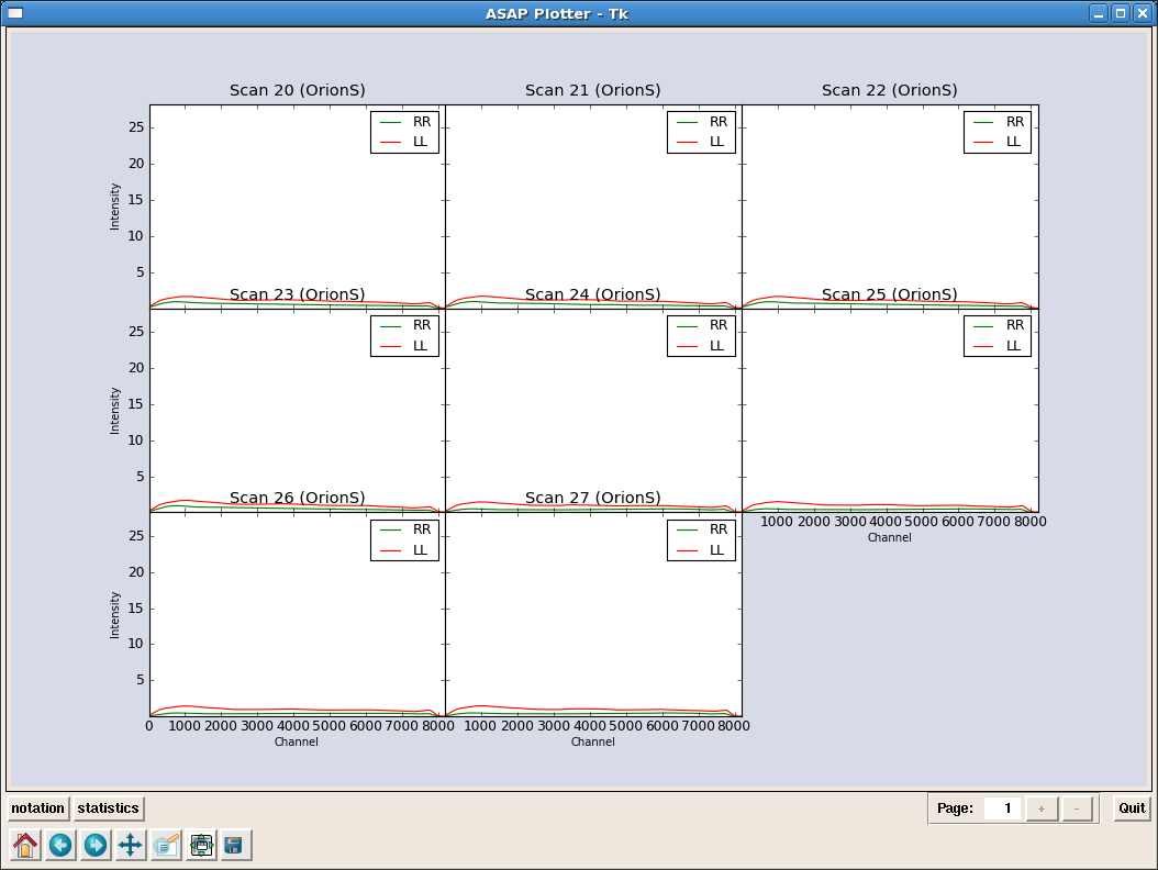
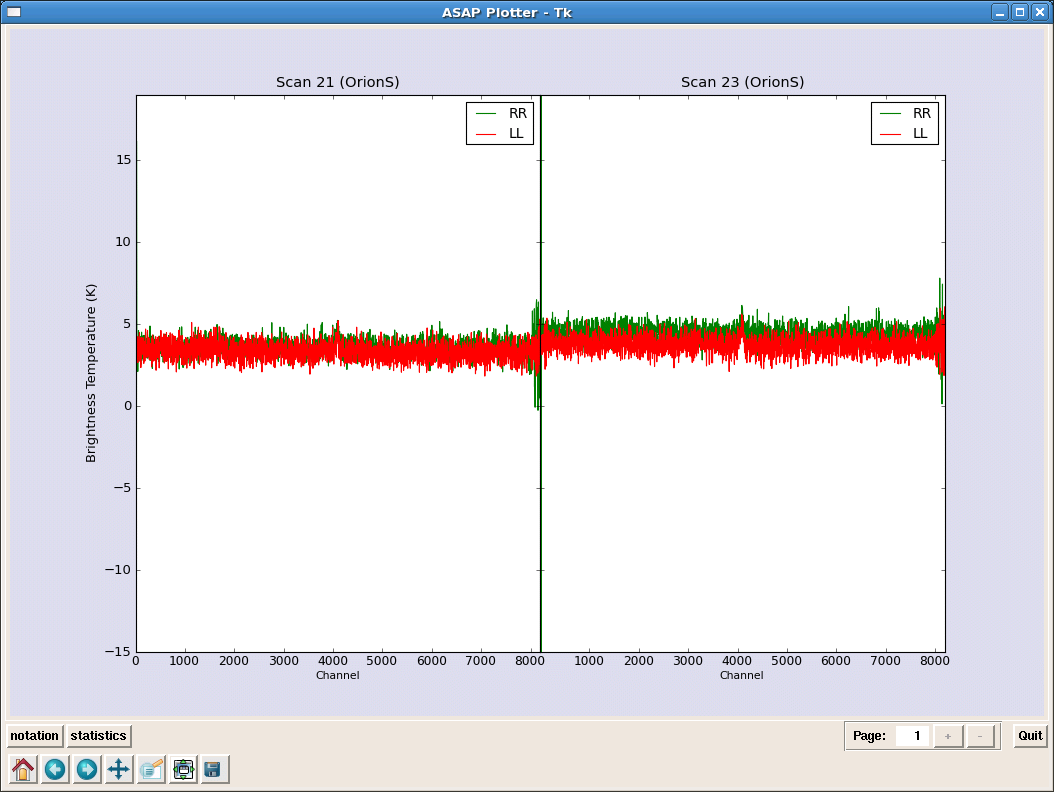
scal=sd.calps(s,[20,21,22,23])          # Calibrate HC3N scans

Figure 8.7: Two panel plot of the calibrated spectra. The GBT data have a separate scan for the SOURCE and REFERENCE positions so scans 20,21,22 and 23 result in these two spectra.

_________________________________________________________________________________________

scal.recalc_azel()                      # recalculate az/el to
scal.opacity(0.09)                      # do opacity correction
sel=sd.selector()                       # Prepare a selection
sel.set_ifs(0)                          # select HC3N IF
scal.set_selection(sel)                 # get this IF
stave=sd.average_time(scal,weight=’tintsys’)    # average in time
spave=stave.average_pol(weight=’tsys’)  # average polarizations;Tsys-weighted (1/Tsys**2) average
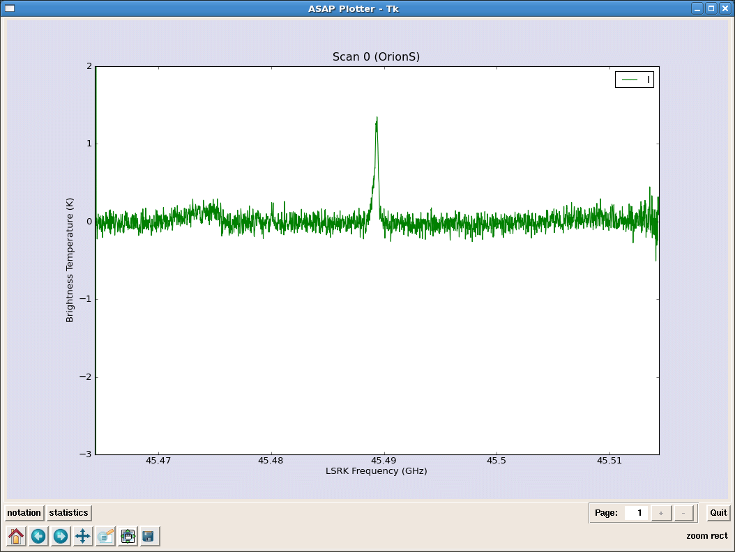
sd.plotter.plot(spave)                  # plot

spave.smooth(’boxcar’,5)                # boxcar 5
spave.auto_poly_baseline(order=2)       # baseline fit order=2
sd.plotter.plot(spave)                  # plot

spave.set_unit(’GHz’)
sd.plotter.plot(spave)
sd.plotter.set_histogram(hist=True)       # draw spectrum using histogram
sd.plotter.axhline(color=’r’,linewidth=2) # zline
sd.plotter.save(’orions_hc3n_reduced.eps’)# save postscript spectrum

Figure 8.8: Calibrated spectrum with a line at zero (using histograms).

_________________________________________________________________________________________

spave.set_unit(’channel’)
rmsmask=spave.create_mask([5000,7000])  # get rms of line free regions
rms=spave.stats(stat=’rms’,mask=rmsmask)#  rms
                                        #----------------------------------------------
                                        #Scan[0] (OrionS_ps) Time[2006/01/19/01:52:05]:
                                        # IF[0] = 0.048
                                        #----------------------------------------------
                                        # LINE
linemask=spave.create_mask([3900,4200])
max=spave.stats(’max’,linemask)         #  IF[0] = 0.918
sum=spave.stats(’sum’,linemask)         #  IF[0] = 64.994
median=spave.stats(’median’,linemask)   #  IF[0] = 0.091
mean=spave.stats(’mean’,linemask)       #  IF[0] = 0.210

                                        # Fitting
spave.set_unit(’channel’)               # set units to channel
sd.plotter.plot(spave)                  # plot spectrum
f=sd.fitter()
msk=spave.create_mask([3928,4255])      # create region around line
f.set_function(gauss=1)                 # set a single gaussian component
f.set_scan(spave,msk)                   # set the data and region for the fitter
f.fit()                                 # fit
f.plot(residual=True)                   # plot residual

f.get_parameters()                      # retrieve fit parameters
#   0: peak = 0.786 K , centre = 4091.236 channel, FWHM = 70.586 channel
#      area = 59.473 K channel
f.store_fit(’orions_hc3n_fit.txt’)      # store fit
# Save the spectrum
spave.save(’orions_hc3n_reduced’,’ASCII’,True)  # save the spectrum

[next] [prev] [prev-tail] [front] [up]

More information about CASA may be found at the CASA web page

This code is available under the terms of the GNU General Public Lincense