Tool
Articles:

Polarimetric
Analysis of
Images

Mosaicwizard

Vis Plane
Calibration
Components

GBT
Observing
Interface

The Image tool is the basic AIPS++ tool with which you manipulate images. Working with it is the Imagepol tool; its job is dedicated polarimetric analysis of images.

Creating Imagepol tools

Here are some examples:

- include 'imagepol.g'
- p1 := imagepol('pks1333.iquv')                 # 1
- im1 := image('pks1333.iquv')                   # 2
- p2 := imagepol(im1)                            # 3
- p2.summary()                                   # 4

The first example makes the Imagepol tool directly from a disk file which has Stokes I, Q, U and V. The second line makes an Image tool from the same file and then we construct the Imagepol tool from that Image tool. We use the summary function of the Imagepol tool to summarise the image (it's just the Image tool function summary that is really invoked).

What can I do with it?

- include 'imagepol.g'
- p := imagepol('pks1333.iquv')    

Recovering specific Stokes

- i := p.stokesi()         # Make Image tools
- v := p.stokesv()
- q := p.stokes('q')
-
- i.statistics()           # Run Image tool functions
- v.view()
- i2 := i.subimage('pks1333.i')  # Copy to disk file 
-
- imagedones()             # Destroy all Image tools when fed up

You can use either the dedicated functions such as stokesi, stokesq or use the stokes function which takes an argument saying which Stokes you want.

Note that the variables i, q and v are in fact Image tools. These Image tools are actually `virtual reference images' (see the August 2000 Newsletter); they reference bits of the image from which the Imagepol tool was originally constructed. You can use all of the Image tool functions on them as usual (a couple of examples are shown).

Generating Secondary Images

- lpi := p.linpolint()           # linearly polarized intensity
- lpa := p.linpolposang()        # linearly polarized position angle 
- tpi := p.totpolint)()          # total polarized intensity 
- flp := p.fraclinpol()          # fractional linear polarization 
- ftp := p.fractotpol()          # fractional total polarization 
- lpi2 := p.pol('lpi')           # Specify which polarized quantity
-
- lpi.statistics()               # Run Image tool function

Again all of the returned variables are virtual Image tools upon which you can run all the Image tool functions.

Generating Error Images

Some of the functions return a scalar (as the error is constant over the image), some return an Image tool.

- sig := p.sigma(clip=5)          # A scalar; best guess at thermal noise 
- sigi := p.sigmastokes('i')      # A scalar; standard deviation of noise
- sigi := p.sigmastokesi();
- sigv := p.sigmastokesv();       # A scalar
-
- siglpi := p.sigmalinpolint()    # A scalar; linearly pol intensity 
- siglpa := p.sigmalinpolposang() # An Image tool; 
                                  # linearly polarized position angle 
- sigflp := p.sigmafraclinpol()   # An Image tool; fractional linear pol 

The philosophy behind the handling of errors is to defer it as long as possible. Many of you are probably familiar with AIPS and Miriad where we blank output images based on a variety of statistical tests. For example, you might blank the linear polarization position angle image when its error is greater than some value. Doing that means you have to keep on regenerating the output image every time you want to try a different blanking value or method.

So to avoid this we have tried to defer this step until you actually use the images. For example

- lpa := p.linpolposang()            # linearly polarized position angle 
- siglpa := p.sigmalinpolposang()    # and its error image
-
- lpa.statistics(mask='$siglpa<10')  # Blank when error > 10 degrees
- lpa.view(mask='$siglpa<20')        # Blank when error > 20 degrees

You can see we have used the mask argument of the statistics and view functions to do this on-the-fly. This is very convenient. Note that we have used the $ syntax (e.g. mask='$siglpa < 20') because the error Image tools are virtual (there is no disk file associated with them); the only way to get at their values is via the tool.

You can of course always copy virtual images to disk if you wish:

- siglpa2 := siglpa.subimage('lpa')
- siglpa2.done()

Finding the Rotation Measure

The Imagepol tool offers you two algorithms. The first is a 'traditional' approach of fitting position angle as a function of frequency. The algorithm used is that of Leahy et al (Astronomy & Astrophysics, 156, 234).

Recall that our Imagepol tool was constructed from an image holding (probably) RA, DEC, Frequency, and Stokes coordinates.

- ok := p.rm(rm='rm', rmerr='rmerr', rmmax=800, maxpaerr=10)

For each spatial pixel, a spectrum (frequency) of position angles is computed (from Q and U stored in the image) and fit. It is very important to specify the rmmax for this algorithm. All RM algorithms of this nature struggle with the n-pi ambiguity and this argument allows you to constrain the process of handling it in some vaguely useful way. We have also specified here a maximum allowed error in the position angle; otherwise that frequency is rejected for that spatial pixel. We output two images, the RM image and its error image. Note that these are disk image files, not virtual images.

- ok := p.rm(rm='rm', rmerr='rmerr', rmmax=800, maxpaerr=10)

The Imagepol tool also offers a new and novel Fourier-based algorithm ( Killeen, Fluke, Zhao and Ekers, 2000, submitted). This algorithm generates an output image which is the polarized intensity as a function of Rotation Measure. It does not suffer from ambiguity and it can recover multiple RM screens unresolved by the beam (as long as they are not along the same line-of-sight).

- p := imagepoltestimage(outfile='iquv.im', rm="1e5 5e5", nx=8, 
+                        ny=8, nf=256, f0=1.4e9, bw=8e6)
- p.frm(amp='amp', pa='pa')   # Fourier transform; 
- amp := image('amp')         # Look at polarized intensity
- amp.view()                  # And reorder to put RM along X-axis

In this example, we have used the other Imagepol constructor imagepoltestimage to generate a test image with the specified Rotation Measure values. The generated test image is 4-dimensional (RA/DEC; 8 by 8 pixels), Stokes (4 pixels; IQUV) and Frequency (256 pixels). The source is just a constant I (if you don't add noise all spatial pixels will be identical) and V. Q and U vary with frequency according to the given Rotation Measures.

The Fourier algorithm Fourier transforms the Complex polarization P = Q + iU image as a function of frequency to a function of Rotation Measure. In the example we save images of the polarized intensity and position angle.

What's missing

Functions for depolarization ratio and errors will also be in place for release 1.5

Tool
Articles:

Polarimetric
Analysis of
Images

Mosaicwizard

Vis Plane
Calibration
Components

GBT
Observing
Interface

Glish, the scripting language and command interpreter for AIPS++, allows the astronomer to have a great deal of control over a series of complex processing steps, running tools and automating decision-making based on the tools' output. But glish also permits astronomical programmers to bundle up their understanding of complex data processing into simple scripts or wizards which are very easy for non-experts to use. Mosaicwizard and imagerwizard, included in release 1.4 of AIPS++, are good examples of the simplicity which can be achieved using glish in this manner.

To start the mosaicwizard, start up AIPS++ and type at the command line:

- include 'mosaicwizard.g';
- mosaicwizard();

Two new windows will appear, one for the mosaicwizard GUI, and one for the scripter, which displays commands emitted by the mosaicwizard.

The mosaicwizard GUI guides you through the mosaicing process, asking for any required information and making reasonable defaults whenever possible. Each step of the process has a title (such as "Select an AIPS++ MeasurementSet or UVFITS file"), along with a few sentences that explain in more depth about what is required and what will be happening. Below the explanatory message there will usually be one or more widgets to accept your input. After you have given your input, the green "Next" button moves you along to the next step. The status line near the bottom of the GUI tells you brief messages about what is going on, such as problems with any input you've given the wizard, or whether an image file has been created or not.

The first step of the mosaicwizard is to select a MeasurementSet or UVFITS file to process. If you don't have one, just leave the input field , and by default AIPS++ will create a MeasurementSet of a seven-pointing VLA D array observation of Cas A at 8 GHz. If you start from a FITS file, as in the case of the Cas A default, handling MeasurementSet arcana will add some extra processing time to a few of the initial steps, so you probably want to keep the MeasurementSet and use it directly in subsequent work with the mosaicwizard. If you already have MeasurementSets in the current directory, click on the wrench icon to the right of the input field, and a file catalog will show you all available MeasurementSets. You can then select a MeasurementSet and click on "send & dismiss" to send the selected MeasurementSet to the mosaicwizard GUI.

The next steps include reading in an optional image that can be used as an initial starting model, selecting the spectral window to image, and selecting the fields you wish to image. after completing this input, you are ready to start thinking about how we want to make our mosaic image.

Because mosaics often have several pointings, cover a large angle on the sky and have many pixels in their final images, and they often reproduce extended structure which takes a long time to deconvolve, mosaics are famous for being slow. However, if you make a small mosaic at low resolution, they aren't slow at all. By default, the mosaicwizard will first make a low resolution image with pixels 4 times larger than full resolution, using only the inner 0.25 of the (u,v) plane. The low resolution mosaic is followed by an intermediate resolution image with pixels 2 times larger than full resolution, using only the inner 0.5 of the (u,v) plane. Finally, a full resolution image is made using all of the (u,v) data. In most cases, the low or intermediate resolution image can be used as a starting model for the next higher resolution image, hence saving on deconvolution time: the high resolution image doesn't need to deconvolve all the flux from scratch, it just needs to incrementally fill in the fine details that were missing from the low resolution model. The first input on the deconvolution page, "(u,v) scaling parameter", controls the maximum baseline used, as a fraction of the maximum baseline present in the MeasurementSet.

In addition to the (u,v) scaling, you can specify the visibility weighting (by the way, when the (u,v) scaling is less than 1.0, a Gaussian taper is also applied in the (u,v) plane so that there is no sharp cutoff in the Fourier plane coverage), the number of Clean or Mem iterations, the deconvolution algorithm (choose between the mfclark, mfhogbom, and mfmultiscale Clean algorithms, or the mfemptiness or mfentropy MEM algorithms), and the presence of a progress display. The multiscale and MEM algorithms require additional input on a supplemental page.

Note that nowhere does the user input the image cell size or the image size. The cell size is set by the reciprocal of the maximum baseline length used for each resolutions' image (divided by 3 for super Nyquist sampling). Initially, the image size is set so that it covers all selected pointings plus half a primary beam's worth of slack on all sides. In later stages, or at higher resolution, the user is invited to generate a mask region which will determine the image size.

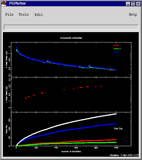
While the low resolution deconvolution is progressing, you may want to focus your attention on the mosaicwizard scripter window showing the most important mosaicing commands, the AIPS++ Log Message window, and the PGPlotter window (only if display progress was invoked) which shows the peak image residual and deconvolved flux as a function of iteration number. Because AIPS++ deconvolves the entire mosaic image with a single approximate PSF, the multifield (ie, mf) algorithms are implemented with a major/minor cycle framework: deconvolution can only proceed so deeply until errors will be made due to the differences between the approximate PSF and the actual PSF for each field. At the end of each cycle, a User Choice window will ask you if you want to proceed with the deconvolution. (If you don't choose after 30 seconds, the default is to continue.) At the start of the next major cycle, the residuals will likely be a bit higher due to errors made from cleaning with an inexact PSF, but these errors are corrected in just a few iterations.

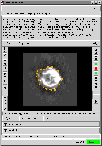
When deconvolution ends (by manually stopping at a major cycle, or by achieving the requested number of iterations), the image is displayed with the viewer, along with instructions for how to create an optional rectangular or polygonal region. This mask region will determine the angular size of the next higher resolution image and will also restrict modeled emission to reside within that region.

When you click on "Next" to leave the viewer, the mosaicwizard leads you back to set the deconvolution parameters once again. The (u,v) scaling has automatically increased by a factor of 2. After you adjust the deconvolution parameters to your liking, you are off making the intermediate resolution image, then inspecting that image with the viewer, perhaps prescribing a new mask. And then on to the full resolution mosaic, and you are finished.

There is nothing special about increasing the resolution in steps of 2. You can jump the (u,v) scaling however you want. You could, of course, make your initial image at full resolution, but I prefer to make my mistakes at low resolution where they aren't quite so glaringly obvious and they don't take so much time.

We are planning a number of enhancements to the mosaicwizard, such as the addition of total power data, dealing with problematic point sources, and handling spectral line data. Look for a more capable version of the mosaicwizard in the release 1.5 of AIPS++.

For more detailed information about the mosaicwizard, see the reference manual under Synthesis:imager:mosaicwizard. For more detailed information about multifield imaging in AIPS++, see the multifield chapter of getting results.

Tool
Articles:

Polarimetric
Analysis of
Images

Mosaicwizard

Vis Plane
Calibration
Components

GBT
Observing
Interface

The previous article in this series provided a description of the Measurement Equation (ME), which is the calibration formalism used in AIPS++. As described in that article, the ME allows antenna-based uv- and image-plane calibration terms, as well as additive and multiplicative baseline-based corrections. This article considers the uv-plane calibration components in more detail for the case of synthesis reduction, and their identification with well-known physical effects.

The antenna-based uv-plane calibration components are represented in the ME by [2,2] Jones matrices, J^vis_i, in a selected polarization representation, using either a circular or linear polarization decomposition. The previous article described how these calibration components are applied in the ME formalism. Further information regarding this formalism can be found in Cornwell (AIPS++ Note 183) and Noordam (AIPS++ Note 182). We enumerate the different types of J^vis_i components here:

• G_i: This diagonal term represents the composite complex electronic gain for all components located after the feed in the signal path.
• B_i: This term denotes the bandpass response, and allows a dependence on frequency in the complex gain terms.
• D_i: This term represents the instrumental polarization response of the feed.
• T_i: This term denotes atmospheric corrections.

The terms listed here can be solved for; there are also two terms of this class in the ME which are either known a priori or pre-computed, namely: C_i, the polarization configuration matrix, which performs polarization conversion operations, and the parallactic angle correction P_i. Note that a subset of the solvable, and non-solvable terms may also may a dependence on angular position, and have image-plane counterparts in the ME to reflect this. The image-plane effects will be the subject of a future article in this series.

The letter designation [G, B, D, T] is used to identify and select calibration component types in the user interface to the imaging and calibration software in AIPS++. The two AIPS++ tools most directly concerned with calibration and imaging are calibrater and imager. The use of these tools is fully described in the AIPS++ cookbook, particularly in the chapters on synthesis calibration and imaging. These chapters detail all the steps required to calibrate and image uv-data, and the associated calibrater and imager tool functions required.

An important point to note is that the tools calibrater and imager represent the uv- and image-plane sides of the Measurement Equation respectively. Therefore imager offers functions concerned with imaging, image-plane calibration components (such as the primary beam correction) and deconvolution, while calibrater is concerned with the application and solution for uv-plane calibration components, as enumerated above. The tools communicate via the MODEL_DATA and CORRECTED_DATA columns in the Measurement Set. The imager tool fills the MODEL_DATA column by integrating across the ME from right to left, starting from the source model or image. For different ways in which to do this see imager.setjy() and imager.ft(). The calibrater tool fills the CORRECTED_DATA column by integrating across the ME from left to right, and applying the known calibration components to the observed data in this process. The associated tool functions for the latter process are calibrater.setapply() and calibrater.correct().

The solvers can form chi squared at any point in the ME at which a calibration component is being solved for; the solvers will be the subject of the next article in this series.

Tool
Articles:

Polarimetric
Analysis of
Images

Mosaicwizard

Vis Plane
Calibration
Components

GBT
Observing
Interface

Several years ago I threw together a prototype graphical interface for the GBT specifically tailored to observers' control of the telescope. This prototype was written in glish/Tk plus a bit of C++, mainly because I was familiar with glish from early aips++ experience. Glish does not benefit from the enormous user community of a language and toolbox like Tcl/Tk, but this does not appear to have been a big disadvantage. Much of the GUI design involved detailed creation of widget combinations at a fairly low level to make optimum use of screen space and quite a bit of widget interconnection to make the GUI respond to interdependent parameters in a way that might be expected by an observer.

The GBT observer interface prototype seemed to fit the requirements of observer's well enough to warrant writing the real interface, now called "GBT Observe," in glish/Tk after a redesign of the code structure. The observer interface now consists of a simulator for each GBT hardware device, written entirely in glish/Tk, a parameter interface to the GBT's monitor and control software, a GUI for interactive observing, and a basic telescope control scripting syntax for programmed observing. The interactive and programmed modes of observing are integrated so that one can use one or the other as appropriate at any given moment. The observing script syntax parser has been written by Darrell Schiebel in C++, and a few utilities and an interface to the JPL solar system ephemeris have also been written in C++. Nearly all of the other code is in glish simply because code development is easier in the interpreted language, and computation efficiency has seldom been an issue.

Telescope observing procedures, from simple tracking and on-offs to raster maps, are written in glish and built into the observer interface. These should suffice for the great majority of GBT observing, but an observer is free to write his or her own procedures using the templates provided. The scripting syntax for programmed observing intentionally excludes arithmetic operators and most flow control to keep the syntax simple. The more powerful language features needed for procedure writing are already available in glish, which most observers will know from their use of aips++.

GBT Observe is still under construction, mostly adding interfaces to the many hardware modules in the system. The core interface to the antenna and a couple of back-ends has been in use for about a year on the GBT mockup in the Jansky lab. A few key interfaces need to be completed in time for GBT commissioning, and detailed control of some of the hardware not normally set up directly by observers will be added as time permits.

A few web documents describing the basic layout from the observer's point of view and the scripting language syntax may be found at

• GBT Observer Interface Prototype
• A Very Brief Introduction to GBT Observing
• GBT Observing Tables
• Writing GBT Procedures in Glish
• Advanced GBT Procedure Writing in Glish

More complete observer documentation is being adapted for the main GBT web pages.

A bit of programmer's documentation on the layout of the code directories and the details of adding a hardware device interface to GBT Observe is posted at

• Adding a device to GBT Observe (programmer's reference)

Since a GBT simulator is part of the observer's interface it should be possible to export the entire interface to a user's home computer for testing observing scripts and user-written procedures before using them on the telescope. We still need to work out the details of exporting the associated C++ glish clients. One way might be to make the interface code part of the aips++ distribution.