National Radio
Astronomy Observatory

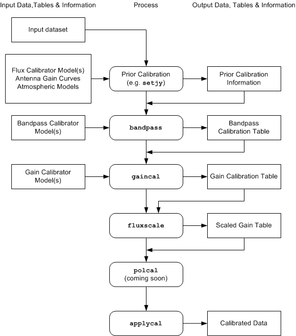
4.2 The Calibration Process — Outline and Philosophy

A work-flow diagram for CASA calibration of interferometry data is shown in Figure 4.1. This should help you chart your course through the complex set of calibration steps. In the following sections, we will detail the steps themselves and explain how to run the necessary tasks and tools.

This can be broken down into a number of discrete phases:

• Calibrator Model Visibility Specification — set model visibilities for calibrators, either unit point source visibilities for calibrators with unknown flux density or structure (generally, sources used for calibrators are approximately point-like), or visibilies derived from a priori images and/or known or standard flux density values.
• Prior Calibration — set up previously known calibration quantities that need to be pre-applied, such antenna gain-elevation curves, atmospheric models, delays, and antenna position offsets. Use the setjy task (§ 4.3.4) for flux densities and models, set the gaincurve (§ 4.3.2) and opacity (§ 4.3.3) parameters in subsequent tasks, and use gencal (§ 4.3.5) for delay and antenna position offsets;
• Bandpass Calibration — solve for the relative gain of the system over the frequency channels in the dataset (if needed), having pre-applied the prior calibration. Use the bandpass task (§ 4.4.2);
• Gain Calibration — solve for the gain variations of the system as a function of time, having pre-applied the bandpass (if needed) and prior calibration. Use the gaincal task (§ 4.4.3);
• Polarization Calibration — solve for polarization leakage terms and linear polarization position angle (§ 4.4.5);
• Establish Flux Density Scale — if only some of the calibrators have known flux densities, then rescale gain solutions and derive flux densities of secondary calibrators. Use the fluxscale task (§ 4.4.4);
• Manipulate, Accumulate, and Iterate — if necessary, accumulate different calibration solutions (tables), smooth, and interpolate/extrapolate onto different sources, bands, and times. Use the accum (§ 4.5.5) and smoothcal (§ 4.5.4) tasks;
• Examine Calibration — at any point, you can (and should) use plotcal (§ 4.5.1) and/or listcal (§ 4.5.2) to look at the calibration tables that you have created;
• Apply Calibration to the Data — this can be forced explicitly by using the applycal task (§ 4.6.1), and can be undone using clearcal (§ 4.6.3);
• Post-Calibration Activities — this includes the determination and subtraction of continuum signal from line data, the splitting of data-sets into subsets (usually single-source), and other operations (such as model-fitting). Use the uvcontsub (§ 4.7.5), split (§ 4.7.1), and uvmodelfit (§ 4.7.7) tasks.

The flow chart and the above list are in a suggested order. However, the actual order in which you will carry out these operations is somewhat fluid, and will be determined by the specific data-reduction use cases you are following. For example, you may need to do an initial Gain Calibration on your bandpass calibrator before moving to the Bandpass Calibration stage. Or perhaps the polarization leakage calibration will be known from prior service observations, and can be applied as a constituent of Prior Calibration.

More information about CASA may be found at the CASA web page

Copyright © 2010 Associated Universities Inc., Washington, D.C.

This code is available under the terms of the GNU General Public Lincense