Interpolation using (accum)

NRAO Home > CASA > CASA Cookbook and User Reference Manual

4.5.5.1 Interpolation using (accum)

Calibration solutions (most notably G or T) can be interpolated onto the timestamps of the science target observations using accum.

The following example uses accum to interpolate an existing table onto a new time grid:

accum(vis=’n4826_16apr.ms’,
      tablein=’’,
      accumtime=20.0,
      incrtable=’n4826_16apr.gcal’,
      caltable=’n4826_16apr.20s.gcal’,
      interp=’linear’,
      spwmap=[0,1,1,1,1,1])

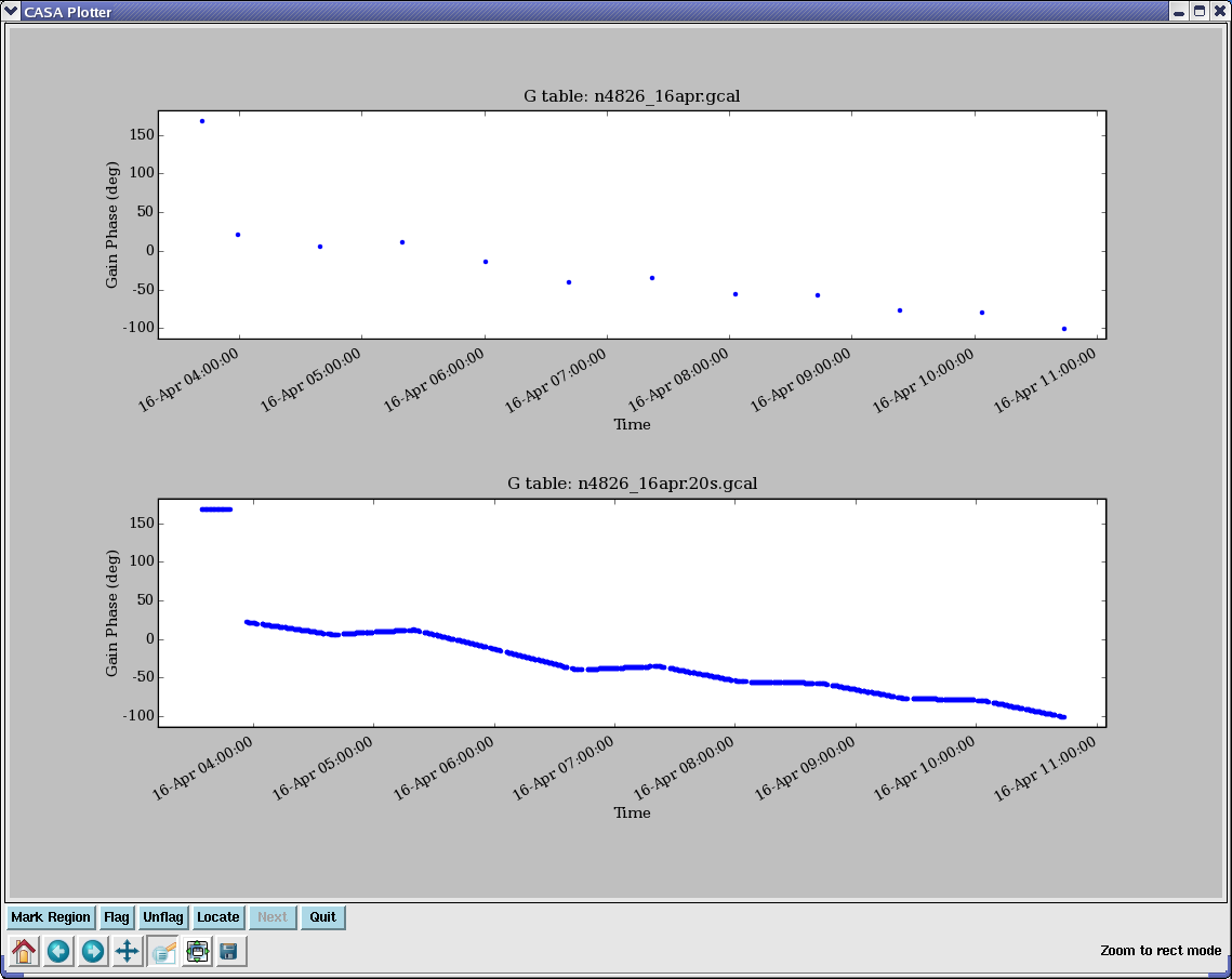
plotcal(’n4826_16apr.gcal’,’’,’phase’,antenna=’1’,subplot=211)
plotcal(’n4826_16apr.20s.gcal’,’’,’phase’,antenna=’1’,subplot=212)

See Figure 4.9 for the plotcal results. The data used in this example is BIMA data (single polarization YY) where the calibrators were observed in single continuum spectral windows (spw=’0,1’) and the target NGC4826 was observed in 64-channel line windows (spw=’2,3,4,5’). Thus, it is necessary to use spwmap=[0,1,1,1,1,1] to map the bandpass calibrator in spw=’0’ onto itself, and the phase calibrator in spw=’1’ onto the target source in spw=’2,3,4,5’.

Figure 4.9: The ’phase’ of gain solutions for NGC4826 before (top) and after (bottom) ’linear’ interpolation onto a 20 sec accumtime grid. The first scan was 3C273 in spw=’0’ while the calibrator scans on 1331+305 were in spw=’1’. The use of spwmap was necessary to transfer the interpolation correctly onto the NGC4826 scans.

_________________________________________________________________________________________

[next] [prev] [prev-tail] [front] [up]

More information about CASA may be found at the CASA web page

This code is available under the terms of the GNU General Public Lincense