 National Radio
Astronomy Observatory
|
|
|||
| NRAO Home > CASA > CASA Cookbook and User Reference Manual |
|
||
4.5.5.2 Incremental Calibration using (accum)
It is occasionally desirable to solve for and apply calibration incrementally. This is the case when a calibration table of a certain type already exists (from a previous solve), a solution of the same type and incremental relative to the first is required, and it is not possible or convenient to recover the cumulative solution by a single solve.
Much of the time, it is, in fact, possible to recover the cumulative solution. This is because the equation describing the solution for the incremental solution (using the original solution), and that describing the solution for their product are fundamentally the same equation—the cumulative solution, if unique, must always be the same no matter what initial solution is. One circumstance where an incremental solution is necessary is the case of phase-only self-calibration relative to a full amplitude and phase calibration already obtained (from a different field).
For example, a phase-only ’G’ self-calibration on a target source may be desired to tweak the full amplitude and phase ’G’ calibration already obtained from a calibrator. The initial calibration (from the calibrator) contains amplitude information, and so must be carried forward, yet the phase-only solution itself cannot (by definition) recover this information, as a full amplitude and phase self-calibration would. In this case, the initial solution must be applied while solving for the phase-only solution, then the two solutions combined to form a cumulative calibration embodying the net effect of both. In terms of the Measurement Equation, the net calibration is the product of the initial and incremental solutions.
Cumulative calibration tables also provide a means of generating carefully interpolated calibration, on variable user-defined timescales, that can be examined prior to application to the data with applycal. The solutions for different fields and/or spectral windows can be interpolated in different ways, with all solutions stored in the same table.
The only difference between incremental and cumulative calibration tables is that incremental tables are generated directly from the calibration solving tasks (gaincal, bandpass, etc), and cumulative tables are generated from other cumulative and incremental tables via accum. In all other respects (internal format, application to data with applycal, plotting with plotcal, etc.), they are the same, and therefore interchangeable. Thus, accumulate and cumulative calibration tables need only be used when circumstances require it.
The accum task represents a generalization on the classic AIPS CLCAL (see sidebox) model of cumulative calibration in that its application is not limited to accumulation of ’G’ solutions. In principle, any basic calibration type can be accumulated (onto itself), as long as the result of the accumulation (matrix product) is of the same type. This is true of all the basic types, except ’D’. Accumulation is currently supported for ’B’, ’G’, and ’T’, and, in future, ’F’ (ionospheric Faraday rotation), delay-rate, and perhaps others. Accumulation of certain specialized types (e.g., ’GSPLINE’, ’TOPAC’, etc.) onto the basic types will be supported in the near future. The treatment of various calibration from ancillary data (e.g., system temperatures, weather data, WVR, etc.), as they become available, will also make use of accumulate to achieve the net calibration.
Note that accumulation only makes sense if treatment of a uniquely incremental solution is required (as described above), or if a careful interpolation or sampling of a solution is desired. In all other cases, re-solving for the type in question will suffice to form the net calibration of that type. For example, the product of an existing ’G’ solution and an amplitude and phase ’G’ self-cal (solved with the existing solution applied), is equivalent to full amplitude and phase ’G’ self-cal (with no prior solution applied), as long as the timescale of this solution is at least as short as that of the existing solution.
One obvious application is to calibrate the amplitudes and phases on different timescales during self-calibration. Here is an example, using the Jupiter VLA 6m continuum imaging example (see Appendix F.2):
ft(vis=’jupiter6cm.usecase.split.ms’,
model=’jupiter6cm.usecase.clean1.model’)
# Phase only self-cal on 10s timescales
gaincal(vis=’jupiter6cm.usecase.split.ms’,
caltable=’jupiter6cm.usecase.phasecal1’,
gaintype=’G’,
calmode=’p’,
refant=’6’,
solint=10.0,
minsnr=1.0)
# Plot up solution phase and SNR
plotcal(’jupiter6cm.usecase.phasecal1’,’’,’phase’,antenna=’1’,subplot=211)
plotcal(’jupiter6cm.usecase.phasecal1’,’’,’snr’,antenna=’1’,subplot=212)
# Amplitude and phase self-cal on scans
gaincal(vis=’jupiter6cm.usecase.split.ms’,
caltable=’jupiter6cm.usecase.scancal1’,
gaintable=’jupiter6cm.usecase.phasecal1’,
gaintype=’G’,
calmode=’ap’,
refant=’6’,
solint=’inf’,
minsnr=1.0)
# Plot up solution amp and SNR
plotcal(’jupiter6cm.usecase.scancal1’,’’,’amp’,antenna=’1’,subplot=211)
plotcal(’jupiter6cm.usecase.scancal1’,’’,’snr’,antenna=’1’,subplot=212)
# Now accumulate these - they will be on the 10s grid
accum(vis=’jupiter6cm.usecase.split.ms’,
tablein=’jupiter6cm.usecase.phasecal1’,
incrtable=’jupiter6cm.usecase.scancal1’,
caltable=’jupiter6cm.usecase.selfcal1’,
interp=’linear’)
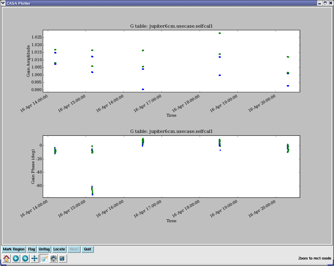
# Plot this up
plotcal(’jupiter6cm.usecase.selfcal1’,’’,’amp’,antenna=’1’,subplot=211)
plotcal(’jupiter6cm.usecase.selfcal1’,’’,’phase’,antenna=’1’,subplot=212)
The final plot is shown in Figure 4.10
_________________________________________________________________________________________
ALERT: Only interpolation is offered in accum, no smoothing (as in smoothcal).
More information about CASA may be found at the
CASA web page
Copyright © 2010 Associated Universities Inc., Washington, D.C.
This code is available under the terms of the GNU General Public Lincense
Home |
Contact Us |
Directories |
Site Map |
Help |
Privacy Policy |
Search