National Radio
Astronomy Observatory

5.3.14 Interactive Cleaning — Example

If interactive=True is set, then an interactive window will appear at various “cycle” stages while you clean, so you can set and change mask regions. These breakpoints are controlled by the npercycle sub-parameter which sets the number of iterations of clean before stopping.

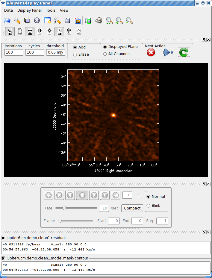
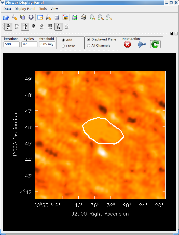
The window controls are fairly self-explanatory. It is basically a form of the viewer. A close-up of the controls are shown in Figure 5.1, and an example can be found in Figures 5.2–5.4. You assign one of the drawing functions (rectangle or polygon, default is rectangle) to the right-mouse button (usually), then use it to mark out regions on the image. Zoom in if necessary (standard with the left-mouse button assignment). Double-click inside the marked region to add it to the mask. If you want to reduce the mask, click the Erase radio button (rather than Add), then mark and select as normal. When finished setting or changing your mask, click the green clockwise arrow “Continue Cleaning” Next Action button. If you want to finish your clean with no more changes to the mask, hit the blue right arrow “Apply mask edits and proceed with non-interactive clean” button. If you want to terminate the clean, click the red X “Stop deconvolving now” button.

While stopped in an interactive step, you can change a number of control parameters in the boxes provided at the left of the menu bar. The main use of this is to control how many iterations before the next breakpoint (initially set to npercycle), how many cycles before completion (initially equal to niter/npercycle), and to change the threshold for ending cleaning. Typically, the user would start with a relatively small number of iterations (50 or 100) to clean the bright emission in tight mask regions, and then increase this as you get deeper and the masking covers more of the emission region. For extended sources, you may end up needing to clean a large number of components (10000 or more) and thus it is useful to set niter to a large number to begin with — you can always terminate the clean interactively when you think it is done. Note that if you change iterations you may also want to change cycles or your clean may terminate before you expect it to.

For strangely shaped emission regions, you may find using the polygon region marking tool (the second from the right in the button assignment toolbar) the most useful.

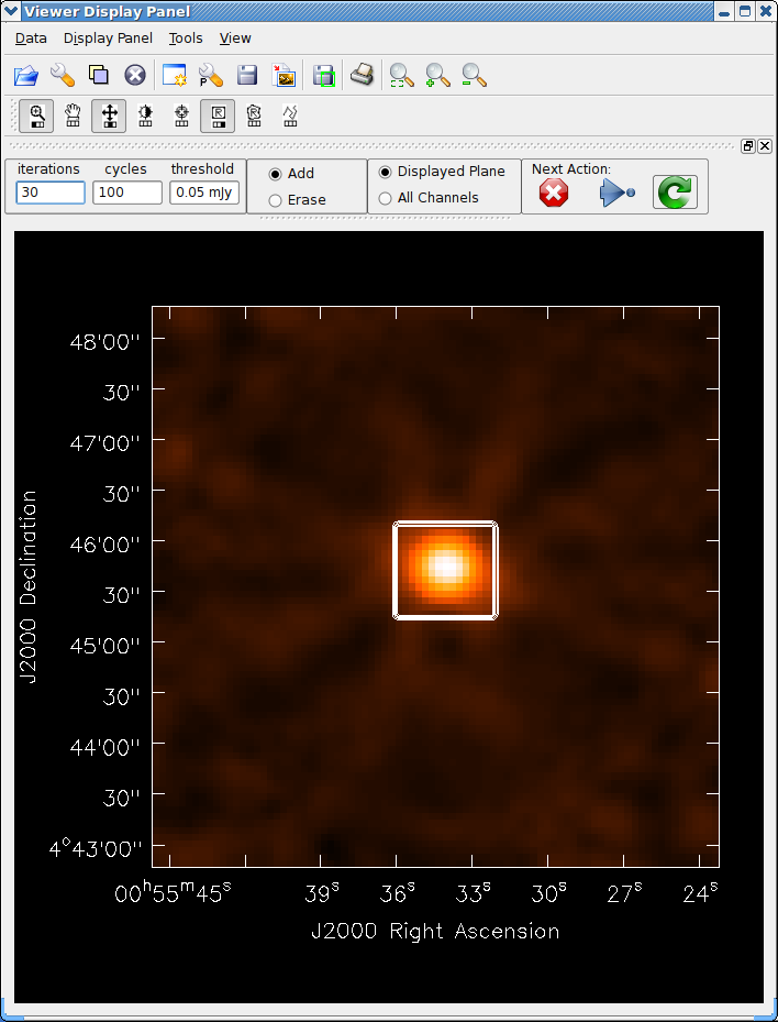
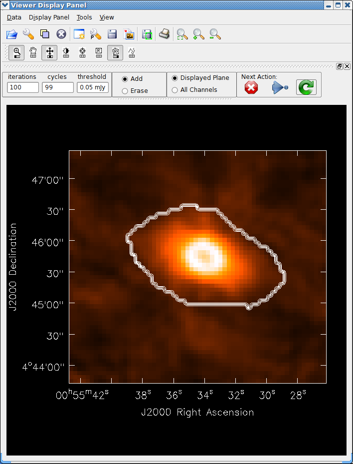
See the example of cleaning and self-calibrating the Jupiter 6cm continuum data given below in Appendix F.2. The sequence of cleaning starting with the “raw” externally calibrated data is shown in Figures 5.2 – 5.4.

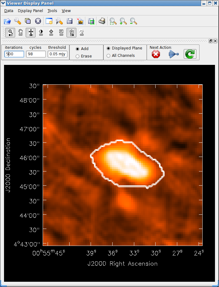
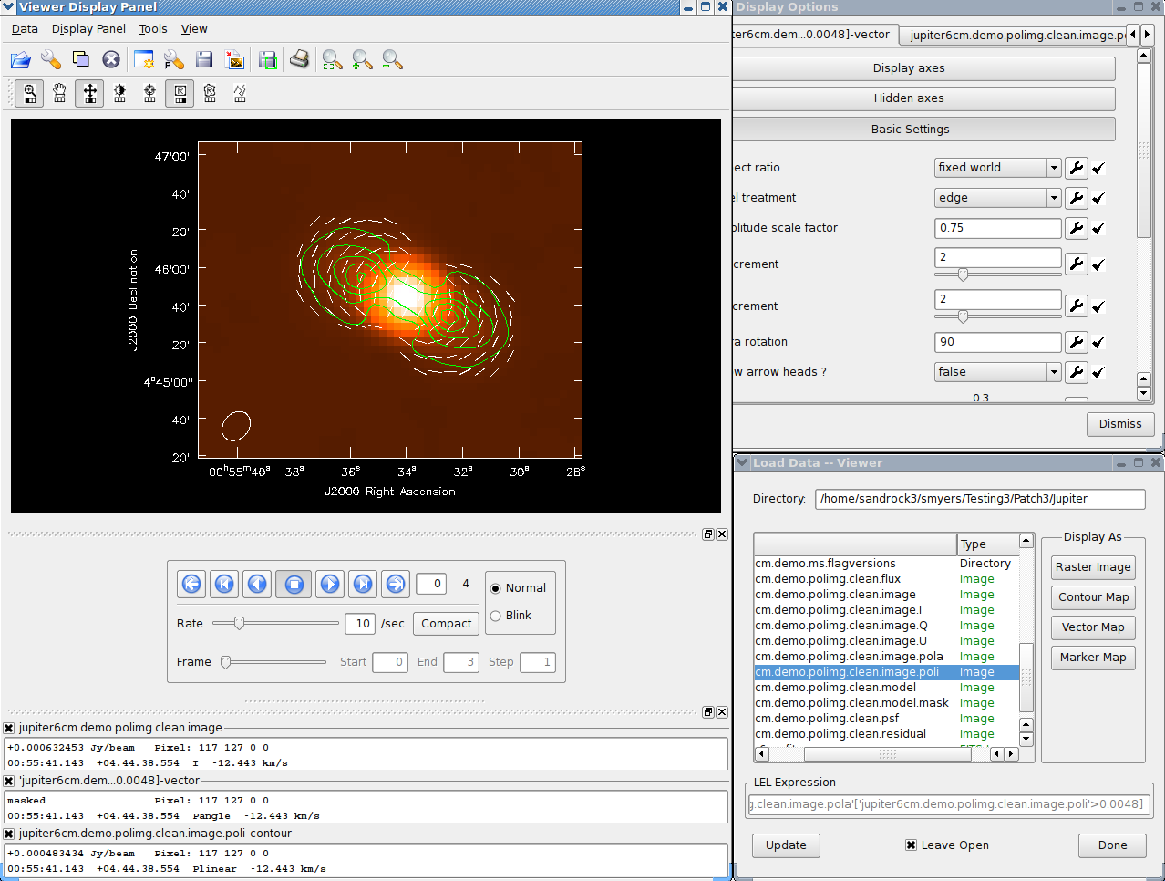
The final result of all this cleaning for Jupiter is shown in Figure 5.5. The viewer (§ 7) was used to overplot the polarized intensity contours and linear polarization vectors calculated using immath (§ 6.5) on the total intensity. See the following chapters on how to make the most of your imaging results.

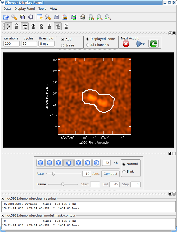
For spectral cube images you can use the tapedeck to move through the channels. You also use the panel with radio buttons for choosing whether the mask you draw applies to the Displayed Plane or to All Channels. See Figure 5.6 for an example. Note that currently the Displayed Plane option is set by default. This toggle is unimportant for single-channel images or mode=’mfs’.

Advanced Tip: Note that while in interactive clean, you are using the viewer. Thus, you have the ability to open and register other images in order to help you set up the clean mask. For example, if you have a previously cleaned image of a complex source or mosaic that you wish to use to guide the placement of boxes or polygons, just use the Open button or menu item to bring in that image, which will be visible and registered on top of your dirty residual image that you are cleaning on. You can then draw masks as usual, which will be stored in the mask layer as before. Note you can blink between the new and dirty image, change the colormap and/or contrast, and carry out other standard viewer operations. See § 7 for more on the use of the viewer.

ALERT: Currently, interactive spectral line cleaning is done globally over the cube, with halts for interaction after searching all channels for the requested npercycle total iterations. It is more convenient for the user to treat the channels in order, cleaning each in turn before moving on. This will be implemented in an upcoming update.

More information about CASA may be found at the CASA web page

Copyright © 2010 Associated Universities Inc., Washington, D.C.

This code is available under the terms of the GNU General Public Lincense