 National Radio
Astronomy Observatory
|
|
|||
| NRAO Home > CASA > CASA Cookbook and User Reference Manual |
|
||
8.2.1.13 sdplot
infile -- name of input SD dataset
antenna -- antenna name or id (only effective for MS input).
fluxunit -- units for line flux
options: ’K’,’Jy’,’’
default: ’’ (keep current fluxunit)
WARNING: For GBT data, see description below.
>>> fluxunit expandable parameter
telescopeparm -- the telescope characteristics
options: (str) name or (list) list of gain info
default: ’’ (none set)
example: if telescopeparm=’’, it tries to get the telescope
name from the data.
Full antenna parameters (diameter,ap.eff.) known
to ASAP are
’ATPKSMB’, ’ATPKSHOH’, ’ATMOPRA’, ’DSS-43’,
’CEDUNA’,’HOBART’. For GBT, it fixes default fluxunit
to ’K’ first then convert to a new fluxunit.
telescopeparm=[104.9,0.43] diameter(m), ap.eff.
telescopeparm=[0.743] gain in Jy/K
telescopeparm=’FIX’ to change default fluxunit
see description below
specunit -- units for spectral axis
options: (str) ’channel’,’km/s’,’GHz’,’MHz’,’kHz’,’Hz’
default: ’’ (=current)
example: this will be the units for masklist
restfreq -- rest frequency used for specunit=’km/s’
default: ’’ (use current setting)
example: 4.6e10 (float value), ’46GHz’ (string with unit)
Allowed units are ’THz’, ’GHz’, ’MHz’, ’kHz’, and ’Hz’
frame -- frequency frame for spectral axis
options: (str) ’LSRK’,’REST’,’TOPO’,’LSRD’,’BARY’,
’GEO’,’GALACTO’,’LGROUP’,’CMB’
default: currently set frame in scantable
WARNING: frame=’REST’ not yet implemented
doppler -- doppler mode
options: (str) ’RADIO’,’OPTICAL’,’Z’,’BETA’,’GAMMA’
default: currently set doppler in scantable
scanlist -- list of scan numbers to process
default: [] (use all scans)
example: [21,22,23,24]
this selection is in addition to field, iflist, pollist,
and beamlist
field -- selection string for selecting scans by name
default: ’’ (no name selection)
example: ’FLS3a*’
this selection is in addition to scanlist, iflist, pollist,
and beamlist
iflist -- list of IF id numbers to select
default: [] (use all IFs)
example: [15]
this selection is in addition to scanlist, field, pollist,
and beamlist
pollist -- list of polarization id numbers to select
default: [] (use all polarizations)
example: [1]
this selection is in addition to scanlist, field, iflist,
and beamlist
beamlist -- list of beam id numbers to select
default: [] (use all beams)
example: [1]
this selection is in addition to scanlist, field, iflist,
and pollist
scanaverage -- average integs within scans
options: (bool) True,False
default: False
timeaverage -- average times for multiple scan cycles
options: (bool) True,False
default: False
example: if True, this happens after calibration
>>>timeaverage expandable parameter
tweight -- weighting for time average
options: ’var’ (1/var(spec) weighted)
’tsys’ (1/Tsys**2 weighted)
’tint’ (integration time weighted)
’tintsys’ (Tint/Tsys**2)
’median’ ( median averaging)
default: ’tintsys’
polaverage -- average polarizations
options: (bool) True,False
default: False
>>>polaverage expandable parameter
pweight -- weighting for polarization average
options: ’var’ (1/var(spec) weighted)
’tsys’ (1/Tsys**2 weighted)
default: ’tsys’
kernel -- type of spectral smoothing
options: ’hanning’,’gaussian’,’boxcar’, ’none’
default: ’none’
>>>kernel expandable parameter
kwidth -- width of spectral smoothing kernel
options: (int) in channels
default: 5
example: 5 or 10 seem to be popular for boxcar
ignored for hanning (fixed at 5 chans)
(0 will turn off gaussian or boxcar)
plottype -- type of plot
options: ’spectra’,’totalpower’,’pointing’,’azel’
default: ’spectra’
>>> plottype expandable parameter
stack -- code for stacking on single plot for spectral plotting
options: ’p’,’b’,’i’,’t’,’s’,’r’ or
’pol’, ’beam’, ’if’, ’time’, ’scan’, ’row’
default: ’p’
example: maximum of 16 stacked spectra
stack by pol, beam, if, time, scan
Note stack selection is ignored when panel=’r’.
panel -- code for splitting into multiple panels for spectral plotting
options: ’p’,’b’,’i’,’t’,’s’,’r’ or
’pol’, ’beam’, ’if’, ’time’, ’scan’, ’row’
default: ’i’
example: maximum of 16 panels
panel by pol, beam, if, time, scan
Note panel selection is ignored when stack=’r’.
flrange -- range for flux axis of plot for spectral plotting
options: (list) [min,max]
default: [] (full range)
example: flrange=[-0.1,2.0] if ’K’
assumes current fluxunit
sprange -- range for spectral axis of plot
options: (list) [min,max]
default: [] (full range)
example: sprange=[42.1,42.5] if ’GHz’
assumes current specunit
linecat -- control for line catalog plotting for spectral plotting
options: (str) ’all’,’none’ or by molecule
default: ’none’ (no lines plotted)
example: linecat=’SiO’ for SiO lines
linecat=’*OH’ for alcohols
uses sprange to limit catalog
WARNING: specunit must be in frequency (*Hz)
to plot from the line catalog!
and must be ’GHz’ or ’MHz’ to use
sprange to limit catalog
linedop -- doppler offset for line catalog plotting (spectral plotting)
options: (float) doppler velocity (km/s)
default: 0.0
example: linedop=-30.0
subplot -- number of subplots (row and column) on a page
NOTICE plotter will slow down when a large number is specified
default: -1 (auto)
example: 23 (2 rows by 3 columns)
colormap -- the colours to be used for plot lines.
default: None
example: colormap="green red black cyan magenta" (html standard)
colormap="g r k c m" (abbreviation)
colormap="#008000 #00FFFF #FF0090" (RGB tuple)
The plotter will cycle through these colours
when lines are overlaid (stacking mode).
linestyles -- the linestyles to be used for plot lines.
default: None
example: linestyles="line dashed dotted dashdot dashdotdot dashdashdot".
The plotter will cycle through these linestyles
when lines are overlaid (stacking mode).
WARNING: Linestyles can be specified only one color has been set.
linewidth -- width of plotted lines.
default: 1
example: linewidth=1 (integer)
linewidth=0.75 (double)
histogram -- plot histogram
options: (bool) True, False
default: False
header -- print header information on the plot
options: (bool) True, False
default: True
The header information is printed only on the logger when
plottype = ’azel’ and ’pointing’.
>>> header expandable parameter
headsize -- header font size
options: (int)
default: 9
plotstyle -- customise plot settings
options: (bool) True, False
default: False
>>> plotstyle expandable parameter
margin -- a list of subplot margins in figure coordinate (0-1),
i.e., fraction of the figure width or height.
The order of elements should be:
[left, bottom, right, top, horizontal space btw panels,
vertical space btw panels]
example: margin = [0.125, 0.1, 0.9, 0.9, 0.2, 0.2]
legendloc -- legend location on the axes (0-10)
options: (integer) 0 -10
see help of "sd.plotter.set_legend" for
the detail of location. Note that 0 (’best’)
is very slow.
default: 1 (’upper right’)
outfile -- file name for hardcopy output
options: (str) filename.eps,.ps,.png
default: ’’ (no hardcopy)
example: ’specplot.eps’,’specplot.png’
Note this autodetects the format from the suffix (.eps,.ps,.png).
overwrite -- overwrite the output file if already exists
options: (bool) True,False
default: False
DESCRIPTION:
Task sdplot displays single-dish spectra or total power data. It assumes that the spectra have been calibrated. It does allow selection of scans, IFs, polarizations, and some time and channel averaging/smoothing options also, but does not write out this data.
*** Only apply to ’spectra’ plottype ***
Note that colormap and linestyles cannot be controlled at a time. The ’linestyles’ is ignored if both of
them are specified. Some plot options, like changing titles, legends, fonts, and the like are
not supported in this task. You should use sd.plotter from the ASAP toolkit directly for
this.
This task uses the JPL line catalog as supplied by ASAP. If you wish to use a different catalog, or have it plot the line IDs from top or bottom (rather than alternating), then you will need to explore the sd toolkit also.
Note that multiple scans and IFs can in principle be handled through stacking and paneling, but this is fairly rudimentary at present and you have little control of what happens in individual panels. We recommend that you use scanlist, field, and iflist to give a single selection for each run.
This task adds an additional toolbar to Matplotlib plotter. See the following instructions for details of its capability.
*** other plottype options ***
Currently most of the parameters are ignored in these modes.
- plottype=’totalpower’ is used to plot the total power data, and only plot option is amplitude versus data row number.
- plottype=’azel’ plots azimuth and elevation tracks of the source.
- plottype=’pointing’ plots antenna poinitings.
See the sdcal description for information on the fluxunit conversion and the telescopeparm parameter. Also, see the sdcal description for note on GBT raw SDFITS format data.
WARNING: be careful plotting otf data with lots of fields!
GUI Plot Control on ASAP Plotter
The principal ways to plot single dish spectra are using the sdplot task and sd.plotter toolkit. These task and toolkit load ASAP Plotter which uses the matplotlib plotting library to display plots. You can find information on matplotlib at http://matplotlib.sourceforge.net/.
_________________________________________________________________________________________
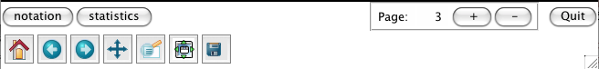
The ASAP Plotter has two rows of buttons at the bottom to control interactive operations as shown in Figure 8.3. When none of the button is depressed, the ASAP Plotter is in spectral value mode. Click on a spectrum to select it and drag the mouse to print the spectral value at the channel position of mouse. The value is printed to the bottom right corner of plotter window.
The buttons on the lower row are the standard matplotlib navigation buttons. See § 3.3.2.1 about details of their capabilities.
In a row above it, there are a set of the other buttons (left to right):
- notation — If depressed lets you edit texts on the plotter. See below for details of text edition. Clicking the button again will un-depress it and go back to the default spectral value mode.
- statistics — If depressed lets you print statics of a selected regions of scantable to the logger. See below for details of region selection. Clicking the button again will un-depress it and go back to the default spectral value mode.
- + and - — Step to the next or previous plot in an iteration. The page counter on their left shows the current page number.
- Quit — Click this to close ASAP Plotter.
Editing texts on the plotter
_________________________________________________________________________________________
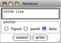
When the notation button is depressed, it lets you edit texts on the plotter. Left-click at a position on the plotter to print a new text, and the Notation window is loaded (Figure 8.4). Type the arbitrary text in the text box, select an anchor, and press the print button to print it at the position you clicked. There are three choices of anchors: figure, panel, and data. The figure or panel locates the text at a fixed position in the figure or subplot, respectively. Its relative position to the figure or subplot boundaries doesn’t change when you resize the plotter. On the other hand, the text is fixed on a position in the data coordinate of subplot, when data is selected as the anchor. The text moves along with plotted spectra as you pan the subplot.
You can modify or delete texts you added on the plotter. To do it, right-click on a text to show a menu with Modify and Delete. When Modify is selected, the Notation window is loaded to modify the selected text. Click on Delete and confirm the operation in a pop-up dialog to delete the text. Clicking the notation button again will un-depress it and go back to the default spectral value mode.
Printing statistics of scantable
When statistics button is depressed, it lets you print statistics of a selected channel region of the
scantable plotted. The statistics values are printed to the logger. You can select a channel region by left-
or right-clicking and dragging the mouse to draw a rectangle. Draw it with left-mouse to print
statistics within the region, while do with right-mouse to print statistics excluding the region.
Clicking the statistics button again will un-depress it and go back to the default spectral value
mode.
More information about CASA may be found at the
CASA web page
Copyright © 2010 Associated Universities Inc., Washington, D.C.
This code is available under the terms of the GNU General Public Lincense
Home |
Contact Us |
Directories |
Site Map |
Help |
Privacy Policy |
Search