Plotting and Editing using plotxy

NRAO Home > CASA > CASA Cookbook and User Reference Manual

3.3.2 Plotting and Editing using plotxy

Inside the Toolkit:

Access to matplotlib is also provided through the pl tool. See below for a description of the pl tool functions.

ALERT: The plotxy code is fragile and slow, and is being replaced by the plotms (§ 3.3.1). We retain plotxy in this release as not all functionality is available yet in plotms.

Plotxy is a tool for visualizing and editing visibility data. Unlike plotms, it is useful in scripting, as it can non-interactively produce a hardcopy plot (see § 3.3.2.13). It also has multi-plot (§ 3.3.2.8), iteration (§ 3.3.2.3), and overplotting (§ 3.3.2.4) functionality—unlike plotms in the current release. Plotxy uses the matplotlib plotting library to display its plots. You can find information on matplotlib at http://matplotlib.sourceforge.net/.

Figure 3.4: The plotxy plotter, showing the Jupiter data versus uv-distance. You can see bad data in this plot. The bottom set of buttons on the lower left are: 1,2,3) Home, Back, and Forward. Click to navigate between previously defined views (akin to web navigation). 4) Pan. Click and drag to pan to a new position. 5) Zoom. Click to define a rectangular region for zooming. 6) Subplot Configuration. Click to configure the parameters of the subplot and spaces for the figures. 7) Save. Click to launch a file save dialog box. The upper set of buttons in the lower left are: 1) Mark Region. Press this to begin marking regions (rather than zooming or panning). 2,3,4) Flag, Unflag, Locate. Click on these to flag, unflag, or list the data within the marked regions. 5) Next. Click to move to the next in a series of iterated plots. Finally, the cursor readout is on the bottom right.

_________________________________________________________________________________________

To bring up this plotter use the plotxy task. The inputs are:

#  plotxy :: X-Y plotter/interactive flagger for visibility data

vis              =         ’’   #  Name of input visibility
xaxis            =     ’time’   #  X-axis: def = ’time’: see help for options
yaxis            =      ’amp’   #  Y-axis: def = ’amp’: see help for options
     datacolumn  =     ’data’   #  data (raw), corrected, model, residual (corrected - model)

selectdata       =      False   #  Other data selection parameters
spw              =         ’’   #  spectral window:channels: ’’==>all, spw=’1:5~57’
field            =         ’’   #  field names or index of calibrators: ’’==>all
averagemode      =         ’’   #  Select averaging type: ’vector’, ’scalar’
restfreq         =         ’’   #  a frequency quanta or transition name. see help for options
extendflag       =      False   #  Have flagging extend to other data points?
subplot          =        111   #  Panel number on display screen (yxn)
plotsymbol       =        ’.’   #  Options include . : , o ^ v > < s + x D d 2 3 4 h H | _
plotcolor        =  ’darkcyn’   #  Plot color
plotrange        = [-1, -1, -1, -1]  #  The range of data to be plotted (see help)
multicolor       =     ’corr’   #  Plot in different colors: Options: none, both, chan, corr
selectplot       =      False   #  Select additional plotting options (e.g, fontsize, title,etc)
overplot         =      False   #  Overplot on current plot (if possible)
showflags        =      False   #  Show flagged data?
interactive      =       True   #  Show plot on gui?
figfile          =         ’’   #  ’’= no plot hardcopy, otherwise supply name
async            =      False   #  If true the taskname must be started using plotxy(...)

ALERT: The plotxy task expects all of the scratch columns to be present in the MS, even if it is not asked to plot the contents. If you get an error to the effect "Invalid Table operation: Table: cannot add a column" then use clearcal() to force these columns to be made in the MS. Note that this will clear anything in all scratch columns (in case some were actually there and being used).

Setting selectdata=True opens up the selection sub-parameters:

selectdata       =       True   #   Other data selection parameters
     antenna     =         ’’   #   antenna/baselines: ’’==>all, antenna = ’3,VA04’
     timerange   =         ’’   #   time range: ’’==>all
     correlation =         ’’   #   correlations: default = ’’
     scan        =         ’’   #   scan numbers: Not yet implemented
     feed        =         ’’   #   multi-feed numbers: Not yet implemented
     array       =         ’’   #   array numbers: Not yet implemented
     uvrange     =         ’’   #   uv range’’==>all; uvrange = ’0~100kl’ (default unit=meters)

These are described in § 2.3.

Averaging is controlled with the set of parameters

averagemode      =   ’vector’   #  Select averaging type: vector, scalar
     timebin     =        ’0’   #  Length of time-interval in seconds to average
     crossscans  =      False   #  Have time averaging cross scan boundaries?
     crossbls    =      False   #  have averaging cross over baselines?
     crossarrays =      False   #  have averaging cross over arrays?
     stackspw    =      False   #  stack multiple spw on top of each other?
     width       =        ’1’   #  Number of channels to average

See § 3.3.2.9 below for more on averaging.

You can extend the flagging beyond the data cell plotted:

extendflag          =   True    #  Have flagging extend to other data points?
     extendcorr     =     ’’    #  flagging correlation extension type
     extendchan     =     ’’    #  flagging channel extension type
     extendspw      =     ’’    #  flagging spectral window extension type
     extendant      =     ’’    #  flagging antenna extension type
     extendtime     =     ’’    #  flagging time extension type

See § 3.3.2.11 below for more on flag extension.

The restfreq parameter can be set to a transition or frequency:

restfreq            =    ’HI’   #  a frequency quanta or transition name. see help for options
     frame          =  ’LSRK’   #  frequency frame for spectral axis. see help for options
     doppler        = ’RADIO’   #  doppler mode. see help for options

See § 3.3.2.12 below for more on setting rest frequencies and frames.

Setting selectplot=True will open up a set of plotting control sub-parameters. These are described in § 3.3.2.2 below.

The interactive and figfile parameters allow non-interactive production of hardcopy plots. See § 3.3.2.13 for more details on saving plots to disk.

The iteration, overplot, plotrange, plotsymbol, showflags and subplot parameters deserve extra explanation, and are described below.

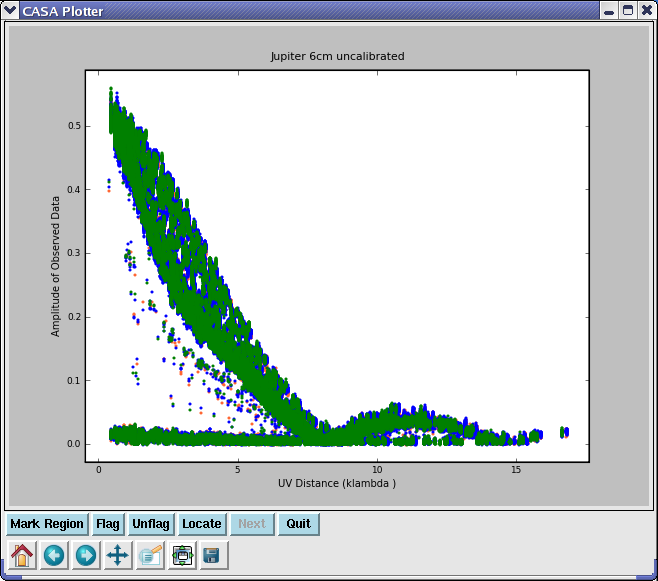
For example:

plotxy(vis=’jupiter6cm.ms’,                # jupiter 6cm dataset
       xaxis=’uvdist’,                     # plot uv-distance on x-axis
       yaxis=’amp’,                        # plot amplitude on y-axis
       field=’JUPITER’,                    # plot only JUPITER
       selectdata=True,                    # open data selection
       correlation=’RR,LL’,                #   plot RR and LL correlations
       selectplot=True,                    # open plot controls
       title = ’Jupiter 6cm uncalibrated’) #   give it a title

The plotter resulting from these settings is shown in figure 3.4.

ALERT: The plotxy task still has a number of issues. The averaging has been greatly speeded up in this release, but there are cases where the plots will be made incorrectly. In particular, there are problems plotting multiple spw at the same time. There are sometimes also cases where data that you have flagged in plotxy from averaged data is done so incorrectly. This task is under active development for the next cycle to fix these remaining problems, so users should be aware of this.

ALERT: Another know problem with (plotxy) is that it fails if the path to your working directory contains spaces in its name, e.g. /users/smyers/MyTest/ is fine, but /users/smyers/My Test/ is not!

   3.3.2.1 GUI Plot Control
   3.3.2.2 The selectplot Parameters
   3.3.2.3 The iteration parameter
   3.3.2.4 The overplot parameter
   3.3.2.5 The plotrange parameter
   3.3.2.6 The plotsymbol parameter
   3.3.2.7 The showflags parameter
   3.3.2.8 The subplot parameter
   3.3.2.9 Averaging in plotxy
   3.3.2.10 Interactive Flagging in plotxy
   3.3.2.11 Flag extension in plotxy
   3.3.2.12 Setting rest frequencies in plotxy
   3.3.2.13 Printing from plotxy
   3.3.2.14 Exiting plotxy
   3.3.2.15 Example session using plotxy

[next] [prev] [prev-tail] [front] [up]

More information about CASA may be found at the CASA web page

This code is available under the terms of the GNU General Public Lincense