Viewing a contour map

NRAO Home > CASA > CASA Cookbook and User Reference Manual

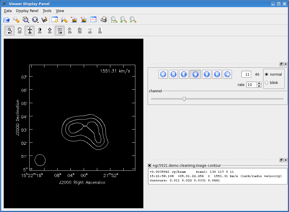
7.3.2 Viewing a contour map

Viewing a contour image is similar to the process above. A contour map shows lines of equal data value (e.g., flux density) for the selected plane of gridded data (Figure 7.10). Contour maps are particularly useful for overlaying on raster images so that two different measurements of the same part of the sky can be shown simultaneously (§ 7.3.3).

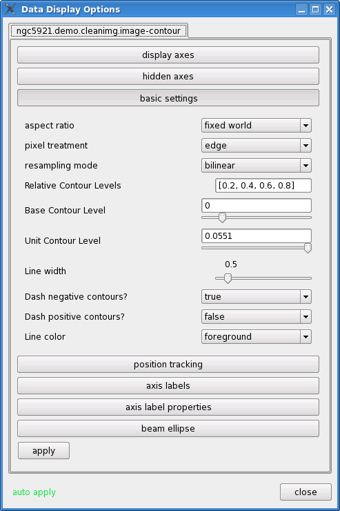
Several basic settings options control the contour levels used. The contours themselves are specified by a list in the box Relative Contour Levels. These are defined relative to the two other parameters, the Base Contour Level (which sets what 0 in the relative contour list corresponds to in the image), and the Unit Contour Level (which sets what 1 in the relative contour list corresponds to in the image). Note that negative contours are usually dashed. ALERT: This scheme was adopted in 2.4.0 and is slightly different to that used in previous versions.

Figure 7.10: The Viewer Display Panel (left) and Data Display Options panel (right) after choosing contour map from the Load Data panel. The image shown is for channel 11 of the NGC5921 cube, selected using the Animator tape deck, and zoomed in using the tool bar icon. Note the different options in the open basic settings category of the Data Display Options panel (as compared to raster image in Figure 7.1).

_________________________________________________________________________________________

For example, it is relatively straightforward to set fractional contours (e.g. “percent levels”), e.g.:

   Relative Contour Levels = [0.2, 0.4, 0.6, 0.8]
   Base Contour Level = 0.0
   Unit Contour Level = <image max>

This maps the maximum to 1 and thus our contours are fractions of the peak.

Another example shows how to set absolute values so that the contours are given in flux density units (Jy):

   Relative Contour Levels = [0.010, 0.0.020, 0.040, 0.080, 0.160, 0.320]
   Base Contour Level = 0.0
   Unit Contour Level = 1.0

Here we have contours starting at 10mJy and doubling every contour.

We can also set contours in multiples of the image rms (“sigma”):

   Relative Contour Levels = [-3,3,5,10,15,20]
   Base Contour Level = 0.0
   Unit Contour Level = <image rms>

Here we have first contours at negative and positive 3-sigma. You can get the image rms using the imstat task (§ 6.7) or using the Viewer statistics tool on a region of the image (§ 7.2.3).

As a final example, not all images are of intensity, for example a moment-1 image (§ 6.6) has units of velocity. In this case, absolute contours will work fine, but by default the viewer will set fractional contours but referred to the min and max velocity:

   Relative Contour Levels = [0.2, 0.4, 0.6, 0.8]
   Base Contour Level = <image min>
   Unit Contour Level = <image max>

Here we have contours spaced evenly from min to max, and this is what you get by default if you load a non-intensity image (like the moment-1 image). See Figure 7.11 for an example of this.

[next] [prev] [prev-tail] [front] [up]

More information about CASA may be found at the CASA web page

This code is available under the terms of the GNU General Public Lincense