POLARISATION COORDINATES

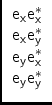
In the 2 x 2 signal domain, the electric field vector $\vec{E}\,$ of the incident plane wave can be represented either in a linear polarisation coordinate frame ( $\sf x$ , $\sf y$ ) or a circular polarisation coordinate frame ( $\sf r$ , $\sf l$ ). Jones matrices are linear operators in the chosen frame:

$\displaystyle \vec{V}^{+}_{{\sf i}}$ = $\displaystyle \left(\vphantom{\begin{array}{c} {\sf v}_{{\sf i}{\sf p}}\\ {\sf v}_{{\sf i}{\sf q}} \end{array}}\right.$ $\displaystyle \begin{array}{c} {\sf v}_{{\sf i}{\sf p}}\\ {\sf v}_{{\sf i}{\sf q}} \end{array}$ $\displaystyle \left.\vphantom{\begin{array}{c} {\sf v}_{{\sf i}{\sf p}}\\ {\sf v}_{{\sf i}{\sf q}} \end{array}}\right)$ = $\displaystyle \sf J^{+}_{{\sf i}}$ $\displaystyle \left(\vphantom{\begin{array}{c} {\sf e}_{{{\sf x}}}\\ {\sf e}_{{{\sf y}}} \end{array}}\right.$ $\displaystyle \begin{array}{c} {\sf e}_{{{\sf x}}}\\ {\sf e}_{{{\sf y}}} \end{array}$ $\displaystyle \left.\vphantom{\begin{array}{c} {\sf e}_{{{\sf x}}}\\ {\sf e}_{{{\sf y}}} \end{array}}\right)$ or $\displaystyle \vec{V}^{\odot}_{{\sf i}}$ = $\displaystyle \sf J^{\odot}_{{\sf i}}$ $\displaystyle \left(\vphantom{\begin{array}{c} {\sf e}_{{\sf r}}\\ {\sf e}_{{\sf l}} \end{array}}\right.$ $\displaystyle \begin{array}{c} {\sf e}_{{\sf r}}\\ {\sf e}_{{\sf l}} \end{array}$ $\displaystyle \left.\vphantom{\begin{array}{c} {\sf e}_{{\sf r}}\\ {\sf e}_{{\sf l}} \end{array}}\right)$

(13)

$\displaystyle \vec{V}^{+}_{{\sf i}{\sf j}}$ = ( $\displaystyle \sf J^{+}_{{\sf i}}$ $\displaystyle \otimes$ $\displaystyle \sf J^{+}_{{\sf j}}^{\ast}$ ) ( $\displaystyle \vec{E}\,$ $\displaystyle \otimes$ $\displaystyle \vec{E}^{\ast}_{}$ ) = ( $\displaystyle \sf J^{+}_{{\sf i}}$ $\displaystyle \otimes$ $\displaystyle \sf J^{+}_{{\sf j}}^{\ast}$ ) $\displaystyle \left(\vphantom{\begin{array}{c} {\sf e}_{{{\sf x}}}{\sf e}_{{{\... ...x}}}^{*} \\ {\sf e}_{{{\sf y}}}{\sf e}_{{{\sf y}}}^{*} \end{array}}\right.$ $\displaystyle \begin{array}{c} {\sf e}_{{{\sf x}}}{\sf e}_{{{\sf x}}}^{*} \\ ... ..._{{{\sf x}}}^{*} \\ {\sf e}_{{{\sf y}}}{\sf e}_{{{\sf y}}}^{*} \end{array}$ $\displaystyle \left.\vphantom{\begin{array}{c} {\sf e}_{{{\sf x}}}{\sf e}_{{{\... ...x}}}^{*} \\ {\sf e}_{{{\sf y}}}{\sf e}_{{{\sf y}}}^{*} \end{array}}\right)$ = ( $\displaystyle \sf J^{+}_{{\sf i}}$ $\displaystyle \otimes$ $\displaystyle \sf J^{+}_{{\sf j}}^{\ast}$ ) $\displaystyle \sf S^{+}_{}$ $\displaystyle \vec{I}\,$ ( $\displaystyle \sf l$ , $\displaystyle \sf m$ )

(14)

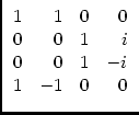
and there is a similar expression for circular polarisation coordinates. Thus, as emphasised in [2], the Stokes vector $\vec{I}\,$ ( $\sf l$ , $\sf m$ ) and the coherency vector $\vec{V}_{{\sf i}{\sf j}}$ represent the same physical quantity, but in different abstract coordinate frames. A `Stokes matrix' $\sf S$ is a coordinate transformation matrix in the 4 x 4 coherency domain: $\sf S^{+}_{}$ transforms the representation from Stokes coordinates (I,Q,U,V) to linear polarisation coordinates ( $\sf x$ $\sf x$ , $\sf x$ $\sf y$ , $\sf y$ $\sf x$ , $\sf y$ $\sf y$ ). 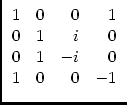Similarly, $\sf S^{\odot}_{}$ transforms to circular polarisation coordinates ( $\sf r$ $\sf r$ , $\sf r$ $\sf l$ , $\sf l$ $\sf r$ , $\sf l$ $\sf l$ ). Following the convention of [4], we write:³

$\displaystyle \sf S^{+}_{}$ = $\displaystyle {\textstyle\frac{1}{2}}$ $\displaystyle \left(\vphantom{\begin{array}{rrrr} 1 & 1 & 0 & 0\\ 0 & 0 & 1 & i\\ 0 & 0 & 1 &-i\\ 1 &-1 & 0 & 0 \end{array}}\right.$ $\displaystyle \begin{array}{rrrr} 1 & 1 & 0 & 0\\ 0 & 0 & 1 & i\\ 0 & 0 & 1 &-i\\ 1 &-1 & 0 & 0 \end{array}$ $\displaystyle \left.\vphantom{\begin{array}{rrrr} 1 & 1 & 0 & 0\\ 0 & 0 & 1 & i\\ 0 & 0 & 1 &-i\\ 1 &-1 & 0 & 0 \end{array}}\right)$ $\displaystyle \sf S^{\odot}_{}$ = $\displaystyle {\textstyle\frac{1}{2}}$ $\displaystyle \left(\vphantom{\begin{array}{rrrr} 1 & 0 & 0 & 1\\ 0 & 1 & i & 0\\ 0 & 1 &-i & 0\\ 1 & 0 & 0 &-1 \end{array}}\right.$ $\displaystyle \begin{array}{rrrr} 1 & 0 & 0 & 1\\ 0 & 1 & i & 0\\ 0 & 1 &-i & 0\\ 1 & 0 & 0 &-1 \end{array}$ $\displaystyle \left.\vphantom{\begin{array}{rrrr} 1 & 0 & 0 & 1\\ 0 & 1 & i & 0\\ 0 & 1 &-i & 0\\ 1 & 0 & 0 &-1 \end{array}}\right)$

(15)

$\sf S$ -matrices are almost unitary, i.e. except for a normalising constant: ( $\sf S$ )^-1 = 2( $\sf S$ )^*T. $\sf S$ cannot be factored into feed-based parts. The two Stokes matrices are related by:

$\displaystyle \cal {H}$ = $\displaystyle {\frac{1}{\sqrt{2}}}$ $\displaystyle \left(\vphantom{\begin{array}{cc}1 & i\\ 1 & -i \end{array}}\right.$ $\displaystyle \begin{array}{cc}1 & i\\ 1 & -i \end{array}$ $\displaystyle \left.\vphantom{\begin{array}{cc}1 & i\\ 1 & -i \end{array}}\right)$ $\displaystyle \cal {H}$ ^-1 = $\displaystyle {\frac{1}{\sqrt{2}}}$ $\displaystyle \left(\vphantom{\begin{array}{cc}1 & 1\\ -i & i \end{array}}\right.$ $\displaystyle \begin{array}{cc}1 & 1\\ -i & i \end{array}$ $\displaystyle \left.\vphantom{\begin{array}{cc}1 & 1\\ -i & i \end{array}}\right)$

(18)

Most Jones matrices will have the same form in both polarisation coordinate frames. But if a Jones matrix is expressed in terms of parameters that are defined in one of the two frames, it will have two different but related forms. This is the case for Faraday rotation $\sf F_{{\sf i}}^{}$ , receptor orientation $\sf P_{{\sf i}}^{}$ , and receptor cross-leakage $\sf D_{{\sf i}}^{}$ , in which the orientation w.r.t. the $\sf x$ , ccY frame plays a role. The two forms of a Jones matrix A can be converted into each other by the coordinate transformation matrix $\cal {H}$ and its inverse:

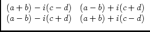
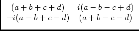
The conversion may be done by hand, using (the elements a, b, c, d may be complex):

$\displaystyle \cal {H}$ $\displaystyle \left(\vphantom{\begin{array}{cc}a & c\\ d & b \end{array}}\right.$ $\displaystyle \begin{array}{cc}a & c\\ d & b \end{array}$ $\displaystyle \left.\vphantom{\begin{array}{cc}a & c\\ d & b \end{array}}\right)$ $\displaystyle \cal {H}$ ^-1 = 0.5 $\displaystyle \left(\vphantom{\begin{array}{cc}(a+b)-i(c-d) & (a-b)+i(c+d)\\ (a-b)-i(c+d) & (a+b)+i(c-d) \end{array}}\right.$ $\displaystyle \begin{array}{cc}(a+b)-i(c-d) & (a-b)+i(c+d)\\ (a-b)-i(c+d) & (a+b)+i(c-d) \end{array}$ $\displaystyle \left.\vphantom{\begin{array}{cc}(a+b)-i(c-d) & (a-b)+i(c+d)\\ (a-b)-i(c+d) & (a+b)+i(c-d) \end{array}}\right)$

(20)

$\displaystyle \cal {H}$ ^-1 $\displaystyle \left(\vphantom{\begin{array}{cc}a & c\\ d & b \end{array}}\right.$ $\displaystyle \begin{array}{cc}a & c\\ d & b \end{array}$ $\displaystyle \left.\vphantom{\begin{array}{cc}a & c\\ d & b \end{array}}\right)$ $\displaystyle \cal {H}$ = 0.5 $\displaystyle \left(\vphantom{\begin{array}{cc}(a+b+c+d) & i(a-b-c+d)\\ -i(a-b+c-d) & (a+b-c-d) \end{array}}\right.$ $\displaystyle \begin{array}{cc}(a+b+c+d) & i(a-b-c+d)\\ -i(a-b+c-d) & (a+b-c-d) \end{array}$ $\displaystyle \left.\vphantom{\begin{array}{cc}(a+b+c+d) & i(a-b-c+d)\\ -i(a-b+c-d) & (a+b-c-d) \end{array}}\right)$

(21)

Applying these general expressions to rotation $\sf Rot$ ( $\alpha$ ) and ellipticity $\sf Ell$ ( $\alpha$ , - $\alpha$ ) matrices (see Appendix for their definition), the conversions are:

$\displaystyle \cal {H}$ $\displaystyle \sf Rot$ ( $\displaystyle \alpha$ ) $\displaystyle \cal {H}$ ^-1	=	$\displaystyle \sf Diag$ (expⁱ, exp^-i)
$\displaystyle \cal {H}$ $\displaystyle \sf Rot$ ( $\displaystyle \alpha$ , $\displaystyle \beta$ ) $\displaystyle \cal {H}$ ^-1	=	see equation
$\displaystyle \cal {H}$ $\displaystyle \sf Ell$ ( $\displaystyle \alpha$ , - $\displaystyle \alpha$ ) $\displaystyle \cal {H}$ ^-1	=	$\displaystyle \sf Rot$ ( $\displaystyle \alpha$ )	(22)

Usually, all matrices in a `Jones chain' will be defined in the same coordinate frame. An exception is the case where linear dipole receptors are used in conjunction with a `hybrid' $\sf H_{{\sf i}}^{}$ to create pseudo-circular receptors:

$\displaystyle \sf J_{{\sf i}}^{}$	=	$\displaystyle \sf G^{\odot}_{{\sf i}}$ $\displaystyle \sf H_{{\sf i}}^{}$ $\displaystyle \sf D^{+}_{{\sf i}}$ $\displaystyle \sf E^{+}_{{\sf i}}$ $\displaystyle \sf P^{+}_{{\sf i}}$ $\displaystyle \sf K^{+}_{{\sf i}}$ $\displaystyle \sf T^{+}_{{\sf i}}$ $\displaystyle \sf F^{+}_{{\sf i}}$ (using $\displaystyle \sf S$ = $\displaystyle \sf S^{+}_{}$ )
	=	$\displaystyle \sf G^{\odot}_{{\sf i}}$ ( $\displaystyle \sf H_{{\sf i}}^{}$ $\displaystyle \sf D^{+}_{{\sf i}}$ $\displaystyle \cal {H}$ ^-1) $\displaystyle \cal {H}$ $\displaystyle \sf E^{+}_{{\sf i}}$ $\displaystyle \sf P^{+}_{{\sf i}}$ $\displaystyle \sf K^{+}_{{\sf i}}$ $\displaystyle \sf T^{+}_{{\sf i}}$ $\displaystyle \sf F^{+}_{{\sf i}}$ (using $\displaystyle \sf S$ = $\displaystyle \sf S^{+}_{}$ )
	=	$\displaystyle \sf G^{\odot}_{{\sf i}}$ $\displaystyle \sf D^{\odot}_{{\sf i}}$ $\displaystyle \cal {H}$ $\displaystyle \sf E^{+}_{{\sf i}}$ $\displaystyle \sf P^{+}_{{\sf i}}$ $\displaystyle \sf K^{+}_{{\sf i}}$ $\displaystyle \sf T^{+}_{{\sf i}}$ $\displaystyle \sf F^{+}_{{\sf i}}$ (using $\displaystyle \sf S$ = $\displaystyle \sf S^{+}_{}$ )
	=	$\displaystyle \sf G^{\odot}_{{\sf i}}$ $\displaystyle \sf D^{\odot}_{{\sf i}}$ $\displaystyle \sf E^{\odot}_{{\sf i}}$ $\displaystyle \sf P^{\odot}_{{\sf i}}$ $\displaystyle \sf K^{\odot}_{{\sf i}}$ $\displaystyle \sf T^{\odot}_{{\sf i}}$ $\displaystyle \sf F^{\odot}_{{\sf i}}$ $\displaystyle \cal {H}$ (using $\displaystyle \sf S$ = $\displaystyle \sf S^{+}_{}$ )
	=	$\displaystyle \sf G^{\odot}_{{\sf i}}$ $\displaystyle \sf D^{\odot}_{{\sf i}}$ $\displaystyle \sf E^{\odot}_{{\sf i}}$ $\displaystyle \sf P^{\odot}_{{\sf i}}$ $\displaystyle \sf K^{\odot}_{{\sf i}}$ $\displaystyle \sf T^{\odot}_{{\sf i}}$ $\displaystyle \sf F^{\odot}_{{\sf i}}$ (using $\displaystyle \sf S$ = $\displaystyle \sf S^{\odot}_{}$ )	(24)

in which $\sf H_{{\sf i}}^{}$ represents an electronic implementation of the coordinate transformation matrix $\cal {H}$ . All these expressions are equivalent in the sense that, in conjunction with the indicated Stokes matrix, they produce a coherency vector in circular polarisation coordinates. The choice of which expression to use depends on whether one wishes to model the feed explicitly in terms of its physical (dipole) properties, or whether one wishes to regard is as a `black box' circular feed with unknown internal structure.

$\displaystyle \cal {H}$ ^-1 $\displaystyle \sf Rot$ ( $\displaystyle \alpha$ ) $\displaystyle \cal {H}$	=	$\displaystyle \sf Ell$ ( $\displaystyle \alpha$ , - $\displaystyle \alpha$ )
$\displaystyle \cal {H}$ ^-1 $\displaystyle \sf Ell$ ( $\displaystyle \alpha$ , - $\displaystyle \alpha$ ) $\displaystyle \cal {H}$	=	$\displaystyle \sf Diag$ (expⁱ, exp^-i)	(23)