Getting Started Documentation Glish Learn More Programming Contact Us
Version 1.9 Build 1556
News FAQ
Search Home

NOTE 224 - AIPS++ Least Squares background

Wim Brouw

22 January 1999

A postscript version of this note is available (124kB).

Contents


Introduction

Trying to find a more stable non-linear least squares method (LSQ) than the one currently used in Newstar, I found another few areas that could be added or improved in the existing routines. In the end I produced a set of routines to handle linear and non-linear cases, both with or without SVD, and constraint equations.

In addition the present document describes the usage and background of the different routines.

Least squares solutions in Aips++ have the following general background:

1.
all are based on creating normal equations from an, initially unknown, number of condition equations
2.
the actual LSQ-object is a symmetric (or Hermitian) matrix
3.
matrix inversions are done using in-place Cholesky methods where possible: it is for standard use the fastest, least memory consuming and a stable method. In cases where the inverse matrix is needed, the method uses resources of the same order as full LU-decomposition (only if explicit constraint equations are present)
4.
input/output to the LSQ-object is done in any precision, internally all calculations are done in double precision
5.
complex numbers are assumed to be contiguous pairs of real numbers with the real part being the first

The following terminology is used throughout:

n
number of unknowns to be solved
m
number of simultaneous knowns
N
number of condition equations
$ \chi^{2}_{}$
merit function
z*
complex conjugate of z
z$\scriptstyle \Re$
real part of z
z$\scriptstyle \Im$
imaginary part of z
x
column vector of unknowns x0,..., xn - 1
ai
vector of factors a0, i,..., an - 1, i in condition equation i
( i = 0,..., N - 1 )
C
the N x n array of condition equations
A
n x n array: normal equations matrix
L
n column vector: right-hand side normal equations
yi
model value for condition equation i ( i = 0,..., N - 1 )
li
measured value for condition equation i ( i = 0,..., N - 1 )
$ \sigma_{i}^{}$
standard deviation for condition equation i ( i = 0,..., N - 1 )
wi
weight for condition equation i ( wi = 1/$ \sigma_{i}^{2}$)
[ab]
shorthand for $ \sum_{i=0}^{N-1}$wiaibi

The condition equations can, with the above definitions, be written in one of the following ways:

ai . x = li   i = 0,..., N - 1 (1)

or as:


$\displaystyle \sum_{k=0}^{n-1}$aikxk = li   i = 0,..., N - 1     (2)

or as:

C . x = l (3)

The normal matrix is defined as:

A = CT . Q-1 . C (4)

resulting in the normal equations:

A . x = L (5)

where L = CT . Q-1 . l and Q is the covariance matrix of the observations. Here only covariance matrices with the same value in each column i (the `weight' wi) are considered.

Linear equations

Real

The merit function we want to minimise is:


$\displaystyle \chi^{2}_{}$ = $\displaystyle \sum_{i=0}^{N-1}$$\displaystyle \left[\vphantom{ \frac{l_{i}-y_{i}}{\sigma_{i}} }\right.$$\displaystyle {\frac{l_{i}-y_{i}}{\sigma_{i}}}$ $\displaystyle \left.\vphantom{ \frac{l_{i}-y_{i}}{\sigma_{i}} }\right]^{2}$     (6)

For the minimum of $ \chi^{2}_{}$ holds:

$\displaystyle {\frac{\partial \chi^{2}}{\partial x_{k}}}$ = 0   k = 0,..., n - 1 (7)

which leads to the following set of normal equations:

$\displaystyle \sum_{i=0}^{N-1}$$\displaystyle {\frac{\left[ l_{i} - y_{i}\right]}{\sigma_{i}^{2}}}$$\displaystyle {\frac{\partial y_{i}}{\partial x_{k}}}$ = 0   k = 0,..., n - 1 (8)

or in matrix form:

$\displaystyle \left(\vphantom{ \begin{array}{cccc}
\left[ a_{0}a_{0}\right] & ...
...n-1}a_{1}\right] &
\cdots & \left[ a_{n-1}a_{n-1}\right]
\end{array} }\right.$$\displaystyle \begin{array}{cccc}
\left[ a_{0}a_{0}\right] & \left[ a_{0}a_{1}...
...left[ a_{n-1}a_{1}\right] &
\cdots & \left[ a_{n-1}a_{n-1}\right]
\end{array}$ $\displaystyle \left.\vphantom{ \begin{array}{cccc}
\left[ a_{0}a_{0}\right] & ...
...n-1}a_{1}\right] &
\cdots & \left[ a_{n-1}a_{n-1}\right]
\end{array} }\right)$ . x = $\displaystyle \left(\vphantom{ \begin{array}{c}
\left[ a_{0}l\right] \\
\left[ a_{1}l\right] \\
\vdots \\
\left[ a_{n-1}l\right]
\end{array} }\right.$$\displaystyle \begin{array}{c}
\left[ a_{0}l\right] \\
\left[ a_{1}l\right] \\
\vdots \\
\left[ a_{n-1}l\right]
\end{array}$ $\displaystyle \left.\vphantom{ \begin{array}{c}
\left[ a_{0}l\right] \\
\left[ a_{1}l\right] \\
\vdots \\
\left[ a_{n-1}l\right]
\end{array} }\right)$ (9)

or:

A . x = L (10)

This symmetric set of equations can be solved, if the matrix is positive definite, i.e. if there are no dependencies between the columns. The solution is given by:

x = A-1 . L (11)


Errors

After solution for the unknowns x, $ \chi^{2}_{}$ as defined in (6) can be directly calculated if we rewrite it as:

$\displaystyle \chi^{2}_{}$ = [ll] - 2$\displaystyle \sum_{k=0}^{n-1}$[akl]xk + $\displaystyle \sum_{i=0}^{N-1}$wiyi2 (12)

Noting that yi = $ \sum_{k=0}^{n-1}$akxk and using equation (9) to note that [ail] = $ \sum_{k=0}^{n-1}$[aiak]xk, we can rewrite (12) as:

$\displaystyle \chi^{2}_{}$ = [ll] - $\displaystyle \sum_{k=0}^{n-1}$xk[akl] (13)

The $ \chi^{2}_{}$ could be used to assess the goodness of fit if the actual $ \sigma_{i}^{}$'s were known, and the errors are normal distributed. In general the actual values of $ \sigma_{i}^{}$ are not known, and often the distribution is not normal (.e.g. if we solve for logarithmic values). An estimate of the standard deviation can be made by:

$\displaystyle \sigma^{2}_{}$ = $\displaystyle {\frac{\left[ \left( l_{i}-y_{i}\right)^{2}\right]}{N-n}}$ (14)

which can be estimated by:

$\displaystyle \sigma_{o}^{2}$ = $\displaystyle {\frac{\chi^{2}}{N-n}}$ (15)

to give `an error per observation'. The `error per unit weight', or the standard deviation, can be expressed as:

$\displaystyle \sigma_{w}^{2}$ = $\displaystyle {\frac{\chi^{2}}{[1]}}$$\displaystyle {\frac{N}{N-n}}$ (16)

The uncertainty in the solution xi can be expressed as:

$\displaystyle \sigma^{2}_{}$$\displaystyle \left(\vphantom{x_{i}}\right.$xi$\displaystyle \left.\vphantom{x_{i}}\right)$ = $\displaystyle \sum_{k=1}^{N-1}$$\displaystyle \sigma_{k}^{2}$$\displaystyle \left(\vphantom{\frac{\partial{x_{i}}}{\partial{y_{k}}}}\right.$$\displaystyle {\frac{\partial{x_{i}}}{\partial{y_{k}}}}$ $\displaystyle \left.\vphantom{\frac{\partial{x_{i}}}{\partial{y_{k}}}}\right)^{2}$ (17)

Since

xi = $\displaystyle \sum_{k=0}^{n-1}$$\displaystyle \left(\vphantom{\mathbf{A}^{-1}}\right.$A-1$\displaystyle \left.\vphantom{\mathbf{A}^{-1}}\right)_{ik}$$\displaystyle \left[\vphantom{a_{k}l}\right.$akl$\displaystyle \left.\vphantom{a_{k}l}\right]$ (18)

we have:

$\displaystyle {\frac{\partial{x_{i}}}{\partial{y_{k}}}}$ = $\displaystyle \sum_{j=0}^{n-1}$$\displaystyle \left(\vphantom{\mathbf{A}^{-1}}\right.$A-1$\displaystyle \left.\vphantom{\mathbf{A}^{-1}}\right)_{ij}$$\displaystyle {\frac{a_{kj}}{\sigma_{k}^{2}}}$ (19)

leading to:

$\displaystyle \sigma^{2}_{}$$\displaystyle \left(\vphantom{x_{i}}\right.$xi$\displaystyle \left.\vphantom{x_{i}}\right)$ = $\displaystyle \sum_{k=0}^{n-1}$$\displaystyle \sum_{l=0}^{n-1}$$\displaystyle \left(\vphantom{\mathbf{A}^{-1}}\right.$A-1$\displaystyle \left.\vphantom{\mathbf{A}^{-1}}\right)_{ik}$$\displaystyle \left(\vphantom{\mathbf{A}^{-1}}\right.$A-1$\displaystyle \left.\vphantom{\mathbf{A}^{-1}}\right)_{il}$$\displaystyle \left[\vphantom{\sum_{j=0}^{N-1}
\frac{a_{kj}a_{lj}}{\sigma_{j}^{2}}}\right.$$\displaystyle \sum_{j=0}^{N-1}$$\displaystyle {\frac{a_{kj}a_{lj}}{\sigma_{j}^{2}}}$ $\displaystyle \left.\vphantom{\sum_{j=0}^{N-1}
\frac{a_{kj}a_{lj}}{\sigma_{j}^{2}}}\right]$ (20)

Doing the sums, this equation reduces to:

$\displaystyle \sigma^{2}_{}$$\displaystyle \left(\vphantom{x_{i}}\right.$xi$\displaystyle \left.\vphantom{x_{i}}\right)$ = $\displaystyle \left(\vphantom{\mathbf{A}^{-1}}\right.$A-1$\displaystyle \left.\vphantom{\mathbf{A}^{-1}}\right)_{ii}$ (21)

If the $ \sigma_{i}^{}$ was not known originally, the estimate of the standard uncertainties in the unknowns x are:

$\displaystyle \sigma$$\displaystyle \left(\vphantom{x_{i}}\right.$xi$\displaystyle \left.\vphantom{x_{i}}\right)$ = $\displaystyle \sigma_{o}^{}$$\displaystyle \sqrt{{\left(\mathbf{A}^{-1}\right)}_{ii}}$ (22)

If the uncertainties in the unknowns are wanted, the inverse matrix A-1 is calculated by backsubstitution of the identity matrix, and the uncertainties by (22).

Complex

The merit function we want to minimise in this case is:

$\displaystyle \chi^{2}_{}$ = $\displaystyle \sum_{i=0}^{N-1}$$\displaystyle \left[\vphantom{ \frac{l_{i}-y_{i}}{\sigma_{i}} }\right.$$\displaystyle {\frac{l_{i}-y_{i}}{\sigma_{i}}}$ $\displaystyle \left.\vphantom{ \frac{l_{i}-y_{i}}{\sigma_{i}} }\right]$$\displaystyle \left[\vphantom{ \frac{l_{i}-y_{i}}{\sigma_{i}} }\right.$$\displaystyle {\frac{l_{i}-y_{i}}{\sigma_{i}}}$ $\displaystyle \left.\vphantom{ \frac{l_{i}-y_{i}}{\sigma_{i}} }\right]^{*}$ (23)

Differentiating $ \chi^{2}_{}$ leads to the following set of normal equations:

$\displaystyle \left(\vphantom{ \begin{array}{cccc}
\left[ a_{0}^{*}a_{0}\right...
...a_{1}\right] &
\cdots & \left[ a_{n-1}^{*}a_{n-1}\right]
\end{array} }\right.$$\displaystyle \begin{array}{cccc}
\left[ a_{0}^{*}a_{0}\right] & \left[ a_{0}^...
...{n-1}^{*}a_{1}\right] &
\cdots & \left[ a_{n-1}^{*}a_{n-1}\right]
\end{array}$ $\displaystyle \left.\vphantom{ \begin{array}{cccc}
\left[ a_{0}^{*}a_{0}\right...
...a_{1}\right] &
\cdots & \left[ a_{n-1}^{*}a_{n-1}\right]
\end{array} }\right)$ . x = $\displaystyle \left(\vphantom{ \begin{array}{c}
\left[ a_{0}^{*}l\right] \\
...
...{*}l\right] \\
\vdots \\
\left[ a_{n-1}^{*}l\right]
\end{array} }\right.$$\displaystyle \begin{array}{c}
\left[ a_{0}^{*}l\right] \\
\left[ a_{1}^{*}l\right] \\
\vdots \\
\left[ a_{n-1}^{*}l\right]
\end{array}$ $\displaystyle \left.\vphantom{ \begin{array}{c}
\left[ a_{0}^{*}l\right] \\
...
...{*}l\right] \\
\vdots \\
\left[ a_{n-1}^{*}l\right]
\end{array} }\right)$ (24)

The normal matrix is Hermitian. It can be solved by Choleski methods. However, internally the matrix is converted to a real form. Although this has an, in general, small memory penalty, it has no influence on CPU time, and makes it possible to use the same routines for complex and real solutions. The conversion to real is done by splitting each element Aij of the normal matrix into A$\scriptstyle \Re$ij + $ \imath$A$\scriptstyle \Im$ij and replacing it by:

Aij = $\displaystyle \left(\vphantom{ \begin{array}{rr}
{A_{ij}}_{\Re} & -{A_{ij}}_{\Im} \\
{A_{ij}}_{\Im} & {A_{ij}}_{\Re}
\end{array} }\right.$$\displaystyle \begin{array}{rr}
{A_{ij}}_{\Re} & -{A_{ij}}_{\Im} \\
{A_{ij}}_{\Im} & {A_{ij}}_{\Re}
\end{array}$ $\displaystyle \left.\vphantom{ \begin{array}{rr}
{A_{ij}}_{\Re} & -{A_{ij}}_{\Im} \\
{A_{ij}}_{\Im} & {A_{ij}}_{\Re}
\end{array} }\right)$ (25)

and simular replacements for the vector elements xi and Li as:

xi = $\displaystyle \left(\vphantom{ \begin{array}{r}
{x_{i}}_{\Re} \\
{x_{i}}_{\Im}
\end{array} }\right.$$\displaystyle \begin{array}{r}
{x_{i}}_{\Re} \\
{x_{i}}_{\Im}
\end{array}$ $\displaystyle \left.\vphantom{ \begin{array}{r}
{x_{i}}_{\Re} \\
{x_{i}}_{\Im}
\end{array} }\right)$ (26)

and:

Li = $\displaystyle \left(\vphantom{ \begin{array}{r}
{L_{i}}_{\Re} \\
{L_{i}}_{\Im}
\end{array} }\right.$$\displaystyle \begin{array}{r}
{L_{i}}_{\Re} \\
{L_{i}}_{\Im}
\end{array}$ $\displaystyle \left.\vphantom{ \begin{array}{r}
{L_{i}}_{\Re} \\
{L_{i}}_{\Im}
\end{array} }\right)$ (27)

Another reason for solving real rather than complex equations is given in the next section.


Separable complex

In cases where both the unknowns x and their complex conjugates x* appear in the condition equations, differentiating the merit function (23) will not produce a symmetric or Hermitian normal matrix, since there exists no linear relation between xi and x*i. We could, of course, solve for 2n complex equations with added constraints that the sum of even and odd unknowns must be real, and their difference imaginary, but this will lead to 4n complex equations.

If, however, we consider each complex unknown as two real unknowns (i.e. xi$\scriptstyle \Re$ and xi$\scriptstyle \Im$) then differentiating (23) produces the following symmetric set of 2n real equations:

$\displaystyle \left(\vphantom{ \begin{array}{ccccc}
{\left[ {a_{0}}^{*}a_{0}\r...
...&
\cdots &
{\left[ {a_{2n-1}}^{*}a_{2n-1}\right]}_{\Re}
\end{array} }\right.$$\displaystyle \begin{array}{ccccc}
{\left[ {a_{0}}^{*}a_{0}\right]}_{\Re} &
{...
...]}_{\Im} &
\cdots &
{\left[ {a_{2n-1}}^{*}a_{2n-1}\right]}_{\Re}
\end{array}$ $\displaystyle \left.\vphantom{ \begin{array}{ccccc}
{\left[ {a_{0}}^{*}a_{0}\r...
...&
\cdots &
{\left[ {a_{2n-1}}^{*}a_{2n-1}\right]}_{\Re}
\end{array} }\right)$ .

  . $\displaystyle \left(\vphantom{ \begin{array}{c}
{x_{0}}_{\Re} \\
{x_{0}}_{\...
...
{x_{1}}_{\Re} \\
\vdots \\
{x_{n-1}}_{\Im} \\
\end{array} }\right.$$\displaystyle \begin{array}{c}
{x_{0}}_{\Re} \\
{x_{0}}_{\Im} \\
{x_{1}}_{\Re} \\
\vdots \\
{x_{n-1}}_{\Im} \\
\end{array}$ $\displaystyle \left.\vphantom{ \begin{array}{c}
{x_{0}}_{\Re} \\
{x_{0}}_{\...
...
{x_{1}}_{\Re} \\
\vdots \\
{x_{n-1}}_{\Im} \\
\end{array} }\right)$ = $\displaystyle \left(\vphantom{ \begin{array}{c}
{\left[ {a_{0}}^{*}l\right]}_{...
... \\
\vdots \\
{\left[ {a_{2n-1}}^{*}l\right]}_{\Im}
\end{array} }\right.$$\displaystyle \begin{array}{c}
{\left[ {a_{0}}^{*}l\right]}_{\Re} \\
{\left...
...t]}_{\Re} \\
\vdots \\
{\left[ {a_{2n-1}}^{*}l\right]}_{\Im}
\end{array}$ $\displaystyle \left.\vphantom{ \begin{array}{c}
{\left[ {a_{0}}^{*}l\right]}_{...
... \\
\vdots \\
{\left[ {a_{2n-1}}^{*}l\right]}_{\Im}
\end{array} }\right)$ (28)

A number of special cases can be distinguished.

In the `normal' complex case (previous section), a2i $ \equiv$ a2i + 1, and (28) reduces to (25).

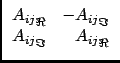
If all a2i and a2i + 1 are real, but specified, e.g., as a complex number, (28) deteriorates into:

$\displaystyle \left(\vphantom{ \begin{array}{ccccc}
\left[ {a_{0}}_{\Re}{a_{0}...
...&
\cdots & \left[ {a_{n-1}}_{\Im}{a_{n-1}}_{\Im} \right]
\end{array} }\right.$$\displaystyle \begin{array}{ccccc}
\left[ {a_{0}}_{\Re}{a_{0}}_{\Re}\right] & ...
...ght] & 0 &
\cdots & \left[ {a_{n-1}}_{\Im}{a_{n-1}}_{\Im} \right]
\end{array}$ $\displaystyle \left.\vphantom{ \begin{array}{ccccc}
\left[ {a_{0}}_{\Re}{a_{0}...
...&
\cdots & \left[ {a_{n-1}}_{\Im}{a_{n-1}}_{\Im} \right]
\end{array} }\right)$ .

  . $\displaystyle \left(\vphantom{ \begin{array}{c}
{x_{0}}_{\Re} \\
{x_{0}}_{\...
...
{x_{1}}_{\Re} \\
\vdots \\
{x_{n-1}}_{\Im} \\
\end{array} }\right.$$\displaystyle \begin{array}{c}
{x_{0}}_{\Re} \\
{x_{0}}_{\Im} \\
{x_{1}}_{\Re} \\
\vdots \\
{x_{n-1}}_{\Im} \\
\end{array}$ $\displaystyle \left.\vphantom{ \begin{array}{c}
{x_{0}}_{\Re} \\
{x_{0}}_{\...
...
{x_{1}}_{\Re} \\
\vdots \\
{x_{n-1}}_{\Im} \\
\end{array} }\right)$ = $\displaystyle \left(\vphantom{ \begin{array}{c}
\left[ {a_{0}}_{\Re}l_{\Re}\ri...
...] \\
\vdots \\
\left[ {a_{n-1}}_{\Im}l_{\Im}\right]
\end{array} }\right.$$\displaystyle \begin{array}{c}
\left[ {a_{0}}_{\Re}l_{\Re}\right] \\
\left[...
...Re}\right] \\
\vdots \\
\left[ {a_{n-1}}_{\Im}l_{\Im}\right]
\end{array}$ $\displaystyle \left.\vphantom{ \begin{array}{c}
\left[ {a_{0}}_{\Re}l_{\Re}\ri...
...] \\
\vdots \\
\left[ {a_{n-1}}_{\Im}l_{\Im}\right]
\end{array} }\right)$ (29)

Note that in this case there is a true separation of the real and imaginary parts of the different unknowns, and two separate real solutions with each n unknowns will produce exactly the same result.

The full and special cases are all catered for in the aips++ routines.

Errors

Using arguments comparable to those in (2.1.1), we can get (13) for the complex case as:

$\displaystyle \chi^{2}_{}$ = [ll*] - $\displaystyle \sum_{k=0}^{n-1}$$\displaystyle \left(\vphantom{ {x_{k}}_{\Re}{\left[ a_{2k}^{*}l \right]}_{\Re} +
{x_{k}}_{\Im}{\left[ a_{2k+1}^{*}l \right]}_{\Im} }\right.$xk$\scriptstyle \Re$$\displaystyle \left[\vphantom{ a_{2k}^{*}l }\right.$a2k*l$\displaystyle \left.\vphantom{ a_{2k}^{*}l }\right]_{\Re}$ + xk$\scriptstyle \Im$$\displaystyle \left[\vphantom{ a_{2k+1}^{*}l }\right.$a2k + 1*l$\displaystyle \left.\vphantom{ a_{2k+1}^{*}l }\right]_{\Im}$$\displaystyle \left.\vphantom{ {x_{k}}_{\Re}{\left[ a_{2k}^{*}l \right]}_{\Re} +
{x_{k}}_{\Im}{\left[ a_{2k+1}^{*}l \right]}_{\Im} }\right)$ (30)

with the a's and x's as defined in (29).

Dependant linear equations

If there are not enough independent condition equations, the normal matrix A cannot be inverted, and a call to WNMLTN will fail with a .false. return value.

The equations could still be solved if some additional `constraint' equations would be introduced. In the more complex cases the precise, let alone the best, form for these additional equations is difficult to determine (e.g. the redundancy situation in Westerbork).

A method known as `Singular value decomposition' (SVD) can be used to obtain the minimal set of orthogonal equations that have to be added to solve the LSQ problem. Several implementations exist in the literature.

In general we can distinguish three types of constrained equations:

All three cases are handled in the LSQ package, the first two in the same way.

The general constraint situation arises from the use of Lagrange multiplicators. Assume that in addition to the condition equations, with measured values, we have a set of p rigorous equations:

$\displaystyle \phi_{i}^{}$(x) = 0   i = 0,..., p - 1 (31)

We must therefore make $ \chi^{2}_{}$ minimal, subject to the set of (31), or:

$\displaystyle \sum_{i=0}^{n-1}$$\displaystyle {\frac{\partial \chi^{2}}{\partial x_{i}}}$dxi = 0 (32)

subject to the conditions:

$\displaystyle \sum_{i=0}^{n-1}$$\displaystyle {\frac{\partial \phi_{k}}{\partial x_{i}}}$dxi = 0   k = 0,..., p - 1 (33)

which leads to a set of n + p equations:

$\displaystyle {\frac{\partial \chi^{2}}{\partial x_{i}}}$ + $\displaystyle \sum_{k=0}^{p-1}$$\displaystyle \lambda_{k}^{}$$\displaystyle {\frac{\partial \phi_{k}}{\partial x_{i}}}$ = 0   i = 0,..., n - 1 (34)

together with the (31).

Note that I have chosen for having constraint equations linear in the unknowns, with a zero value. In cases where this is not adequate (e.g. x + y + z = 360) a simple linear transformation will suffice to make it e.g. x' + y' + z' = 0.

Defining the second term in (34) as Bik, we can write our expanded set of normal equations as:

$\displaystyle \left(\vphantom{\begin{array}{cc}
\mathbf{A} & \mathbf{B} \\
\mathbf{B}^{T} & 0
\end{array} }\right.$$\displaystyle \begin{array}{cc}
\mathbf{A} & \mathbf{B} \\
\mathbf{B}^{T} & 0
\end{array}$ $\displaystyle \left.\vphantom{\begin{array}{cc}
\mathbf{A} & \mathbf{B} \\
\mathbf{B}^{T} & 0
\end{array} }\right)$$\displaystyle \left(\vphantom{\begin{array}{c}
\mathbf{x} \\
\mathbf{\lambda}
\end{array} }\right.$$\displaystyle \begin{array}{c}
\mathbf{x} \\
\mathbf{\lambda}
\end{array}$ $\displaystyle \left.\vphantom{\begin{array}{c}
\mathbf{x} \\
\mathbf{\lambda}
\end{array} }\right)$ = $\displaystyle \left(\vphantom{ \begin{array}{c}
\mathbf{L} \\
0
\end{array}}\right.$$\displaystyle \begin{array}{c}
\mathbf{L} \\
0
\end{array}$ $\displaystyle \left.\vphantom{ \begin{array}{c}
\mathbf{L} \\
0
\end{array}}\right)$ (35)

Unknown constraints

The routines to handle this situation use a method based on ``Pseudo-inverse berekening en Cholesky factorisatie'', Hans van der Marel, 27 maart 1990, Faculty of Geodesy, Delft University. I will briefly describe Hans' paper, together with the additions I have made.

In the case we are considering, the normal equation A has not full column rank. Therefore, there exists, if the rank defect is p, an n x p matrix G, a basis for the null-space of A, with AG = 0. If we assume that B has just sufficient constraint equations to solve the rank defect, the inverse of the matrix in (35) is:
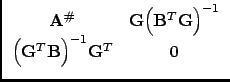
$\displaystyle \left(\vphantom{\begin{array}{cc}
\mathbf{A} & \mathbf{B} \\
\mathbf{B}^{T} & 0
\end{array} }\right.$$\displaystyle \begin{array}{cc}
\mathbf{A} & \mathbf{B} \\
\mathbf{B}^{T} & 0
\end{array}$ $\displaystyle \left.\vphantom{\begin{array}{cc}
\mathbf{A} & \mathbf{B} \\
\mathbf{B}^{T} & 0
\end{array} }\right)^{-1}$ = $\displaystyle \left(\vphantom{\begin{array}{cc}
\mathbf{A}^{\char93 } &
\math...
...ft(\mathbf{G}^{T}\mathbf{B}\right)}^{-1}\mathbf{G}^{T} & 0
\end{array}}\right.$$\displaystyle \begin{array}{cc}
\mathbf{A}^{\char93 } &
\mathbf{G} {\left(\ma...
...
{\left(\mathbf{G}^{T}\mathbf{B}\right)}^{-1}\mathbf{G}^{T} & 0
\end{array}$ $\displaystyle \left.\vphantom{\begin{array}{cc}
\mathbf{A}^{\char93 } &
\math...
...ft(\mathbf{G}^{T}\mathbf{B}\right)}^{-1}\mathbf{G}^{T} & 0
\end{array}}\right)$ (36)

with A# the pseudo-inverse of A. A number of relations hold for A#, the most important for us that BTA# = 0 and A#B = 0, or B is a base for the null-space of A#. For a mininorm solution we can choose B = G. In that case A# is the Moore-Penrose inverse, and BTG is regular and symmetric.

We can now proceed in the following way:

1.
Do a Cholesky factorisation of the normal equations A until the remaining columns of A are dependent. Pivoting along the diagonal of A occurs to make sure that A can be partitioned in an independent and a dependent part with rank defect n2. Dependency is determined by looking at the angle between a column and the space formed by the already determined independent space (the so-called `collinearity number').

If n1 = n - n2, we can say that after n1 Choleski steps, we have:

A = $\displaystyle \left(\vphantom{ \begin{array}{cc}
A_{11} & A_{12} \\
A_{21} & A_{22}
\end{array} }\right.$$\displaystyle \begin{array}{cc}
A_{11} & A_{12} \\
A_{21} & A_{22}
\end{array}$ $\displaystyle \left.\vphantom{ \begin{array}{cc}
A_{11} & A_{12} \\
A_{21} & A_{22}
\end{array} }\right)$ = $\displaystyle \left(\vphantom{ \begin{array}{cc}
U_{11}^{T} & 0 \\
U_{12}^{T} & I
\end{array} }\right.$$\displaystyle \begin{array}{cc}
U_{11}^{T} & 0 \\
U_{12}^{T} & I
\end{array}$ $\displaystyle \left.\vphantom{ \begin{array}{cc}
U_{11}^{T} & 0 \\
U_{12}^{T} & I
\end{array} }\right)$ . $\displaystyle \left(\vphantom{ \begin{array}{cc}
U_{11} & U_{12} \\
0 & \overline{A}_{22}
\end{array} }\right.$$\displaystyle \begin{array}{cc}
U_{11} & U_{12} \\
0 & \overline{A}_{22}
\end{array}$ $\displaystyle \left.\vphantom{ \begin{array}{cc}
U_{11} & U_{12} \\
0 & \overline{A}_{22}
\end{array} }\right)$ (37)

with U11 the Cholesky factor of A11, U12 = U11T-1A12 and $ \overline{A}_{22}^{}$ = A22 - U12TU12.

The collinearity angle $ \delta$ can be determined for the current column i by: sin2$ \delta$ = uii2/aii.

2.
Determine a G1 replacing the (rectangular) U12 from U11G1 = - U12.
3.
Determine a (symmetric) G2 replacing A22 from the rank basis I + G1TG1 = (G2T - 1)(G2 - 1)
4.
determine constraint equations G = $ \left(\vphantom{ G_{1}G_{2},G_{2}}\right.$G1G2, G2$ \left.\vphantom{ G_{1}G_{2},G_{2}}\right)^{T}$.
5.
Solve for the n1 independent unknowns x1 using A11 and L1 by back substitution
6.
Solve constraint equations for the remaining n2 unknowns, using G2 by back substitution: x2 = - G2-1G1Tx1
7.
Make Baarda's S-transform of independent n1 unknowns: x1 = x1 + G1x2.
Setting F = A1-1L1, D = - G2-1G1T and E = $ \left(\vphantom{\begin{array}{c}\mathbf{I}_{n_{1}}+G_{1}\mathbf{D} \\
\mathbf{D} \end{array}}\right.$$ \begin{array}{c}\mathbf{I}_{n_{1}}+G_{1}\mathbf{D} \\
\mathbf{D} \end{array}$ $ \left.\vphantom{\begin{array}{c}\mathbf{I}_{n_{1}}+G_{1}\mathbf{D} \\
\mathbf{D} \end{array}}\right)$, we can write the above steps as:

$\displaystyle \left(\vphantom{\begin{array}{c}
\mathbf{x}_{1} \\  \mathbf{x}_{2}
\end{array}}\right.$$\displaystyle \begin{array}{c}
\mathbf{x}_{1} \\  \mathbf{x}_{2}
\end{array}$ $\displaystyle \left.\vphantom{\begin{array}{c}
\mathbf{x}_{1} \\  \mathbf{x}_{2}
\end{array}}\right)$ = $\displaystyle \left(\vphantom{\begin{array}{c}
\mathbf{I}_{n_{1}}+G_{1}\mathbf{D} \\  \mathbf{D}
\end{array}}\right.$$\displaystyle \begin{array}{c}
\mathbf{I}_{n_{1}}+G_{1}\mathbf{D} \\  \mathbf{D}
\end{array}$ $\displaystyle \left.\vphantom{\begin{array}{c}
\mathbf{I}_{n_{1}}+G_{1}\mathbf{D} \\  \mathbf{D}
\end{array}}\right)$$\displaystyle \left(\vphantom{\begin{array}{c}
A_{1}^{-1}L_{1}
\end{array}}\right.$$\displaystyle \begin{array}{c}
A_{1}^{-1}L_{1}
\end{array}$ $\displaystyle \left.\vphantom{\begin{array}{c}
A_{1}^{-1}L_{1}
\end{array}}\right)$ = E . F (38)

Errors

Errors are determined in the same way as described in (2.1.1), where it should be noted that (13) can either be used summing over n1 variables and using the first guess of x1, or over n and using the final x. Internally the first option is used. The uncertainties in x are determined by calculating the covariance matrix. Using similar arithmetic as in (2.1.1), it can be shown that:

A-1 = E . a1-1 . ET (39)

A-1 is calculated by first solving H = E$ \left(\vphantom{\mathbf{A}_{1}^{-1}
\cdot\mathbf{I}_{n_{1}}}\right.$A1-1 . In1$ \left.\vphantom{\mathbf{A}_{1}^{-1}
\cdot\mathbf{I}_{n_{1}}}\right)$ and then A-1 = E . HT.

Known constraints

In the case of known constraints, hence when B is known in (35), this equation can be solved. Cholesky decomposition does not work in this case, and a, transparent, Crout LU decomposition is done to determine the (symmetric) covariance (i.e. inverse) matrix of the left hand side of (35). .

Errors

Errors are determined as explained in (2.1.1). Since all constraint equations are $ \equiv$ 0, the sum in (13) is taken over n, not over n + p if p are the number of constraint equations.

Non-linear equations

In the case of non-linear condition equations, no simple solution to minimise the merit function (e.g. (6)) exists. A simple solution is to take the condition equation, make a first order Taylor expansion around an estimated $ \hat{\mathbf{x}}$; solve for dx, and iterate till solution found.

However, better and more stable methods exist (e.g. steepest-descend) for some circumstances. A method that seems to be quite stable and using both steepest-descent and Taylor expansion, is the method by Levenberg-Marquardt (see e.g. ``Numerical recipes'', W.H. Press et al., Cambridge University Press).

If we have an estimate for x, we can find a better one by:

$\displaystyle \hat{\mathbf{x}}_{next}^{}$ = $\displaystyle \hat{\mathbf{x}}$ + H-1 . $\displaystyle \left[\vphantom{ -\nabla\chi^{2}(\hat{\mathbf{x}})}\right.$ - $\displaystyle \nabla$$\displaystyle \chi^{2}_{}$($\displaystyle \hat{\mathbf{x}}$)$\displaystyle \left.\vphantom{ -\nabla\chi^{2}(\hat{\mathbf{x}})}\right]$ (40)

where H is the Hessian matrix of $ \chi^{2}_{}$. If our approximation is not good enough, we could use the steepest-descent by calculating:

$\displaystyle \hat{\mathbf{x}}_{next}^{}$ = $\displaystyle \hat{\mathbf{x}}$ - constant . $\displaystyle \left[\vphantom{ -\nabla\chi^{2}(\hat{\mathbf{x}})}\right.$ - $\displaystyle \nabla$$\displaystyle \chi^{2}_{}$($\displaystyle \hat{\mathbf{x}}$)$\displaystyle \left.\vphantom{ -\nabla\chi^{2}(\hat{\mathbf{x}})}\right]$ (41)

The Hessian matrix H has as elements:

Hij = $\displaystyle {\frac{\partial^{2}\chi^{2}}{\partial x_{i}\partial x_{j}}}$ = 2$\displaystyle \sum_{k=0}^{N-1}$$\displaystyle {\frac{1}{\sigma_{i}^{2}}}$$\displaystyle \left[\vphantom{
\frac{\partial y_{k}}{\partial x_{i}}
\frac{\p...
...}-y_{i}\right)
\frac{\partial^{2}y_{i}}{\partial x_{i} \partial x_{j}}}\right.$$\displaystyle {\frac{\partial y_{k}}{\partial x_{i}}}$$\displaystyle {\frac{\partial y_{k}}{\partial x_{j}}}$ - $\displaystyle \left(\vphantom{ l_{i}-y_{i}}\right.$li - yi$\displaystyle \left.\vphantom{ l_{i}-y_{i}}\right)$$\displaystyle {\frac{\partial^{2}y_{i}}{\partial x_{i} \partial x_{j}}}$ $\displaystyle \left.\vphantom{
\frac{\partial y_{k}}{\partial x_{i}}
\frac{\p...
...}-y_{i}\right)
\frac{\partial^{2}y_{i}}{\partial x_{i} \partial x_{j}}}\right]$ (42)

By dropping the second term in (42), and multiplying each Hii term with (1 + $ \lambda$), and defining the first derivative of $ \chi^{2}_{}$ as b, we can combine the equations (40), (41) into:

H . dx = b (43)

which can be solved as standard normal equations.

Choosing $ \lambda$ is the crux of the matter, and where to stop iterating. A start value of $ \lambda$ = 0.001 is used in the following routines. The method looks at the $ \chi^{2}_{}$ for $ \hat{\mathbf{x}}$ + dx. If it has increased over the value of $ \chi^{2}_{}$ for $ \hat{\mathbf{x}}$, $ \hat{\mathbf{x}}$ is unchanged, and $ \lambda$ = 10$ \lambda$. If there is a decrease; a new value for $ \hat{\mathbf{x}}$ is used, and $ \lambda$ = $ \lambda$/10. Iteration can be stopped if the fractional decrease in $ \chi^{2}_{}$ is small (say < 0.001); never if there is an increase in $ \chi^{2}_{}$.

Errors

Errors are calculated as described in (2.1.1). The errors returned by WNMLSN are, of course, only approximations, since the original equations are non-linear, but give a good impression of the residuals. The covariance matrix should be calculated by doing a final linear run on the residuals, and solve the equations.

Summary

An LSQ-object takes a total space of:

9 + (administration)  
(n + p)(n + p + 1)/2 + (normal array)  
4m + (error calculations)  
m(m + p) + (known sides)  
(n + p + 1)/2 + (pivot area)  
(n + p)   (solution) 8 byte words (44)

where n is the number of unknowns (2n if complex); m the number of simultaneously to be solved equations; p the number of external constraint equations. In the non-linear case two LSQ-objects are used. In cases where the inverted normal array is calculated (known constraints) a temporary storage of n2 8-byte words is used.

The following calls are available:

1.
To be given


wnb, October 15, 2006


next up previous home.gif
Please send questions or comments about AIPS++ to aips2-request@nrao.edu.
Copyright © 1995-2000 Associated Universities Inc., Washington, D.C.

Return to AIPS++ Home Page
2006-10-15