Version 1.8 Build 235

News	FAQ
Search	Home

Next: 8. Arecibo Observatory Spectral Line Reduction with DISH Up: Volume 3 - Telescope Specific Processing Previous: 6. Parkes Multibeam Reduction

Subsections

7. Reducing JCMT data in DISH

R. Phillips & J. McMullin

7.1 Setting Your Environment

7.1.1 Starting AIPS++

To start AIPS++, issue the following commands (from the bash shell):

> . /aips++/stable/aipsinit.sh
> aips++

7.1.2 Making AIPS++ run faster

Here are several hints for speeding up your performance, if the operation/startup of AIPS++ seems sluggish.

Store cache files on the computer you run from by adding the following line to your .aipsrc file:

	user.aipsdir: /tmp/username_aips++

	where username is your username, e.g.,
	user.aipsdir: /tmp/rphillips_aips++

If you do not want to have the toolmanager GUI available on starting AIPS++, you can suppress it and speed up the startup time by including the following lines in your .aipsrc file:
```
	toolmanager.fullgui: F
	toolmanager.gui.auto: F
```
The toolmanager isn't directly needed for any DISH operations. Should you want it, it can be used at a later time by typing:
```
	tm.gui();
```
Run AIPS++ from the computer which hosts the disks with your data. Typically the data I/O over NFS is slow and the above bypasses this as much as possible

AIPS++ builds its cache file structure the first time it is started with a new user.aipsdir, and each time you start a new version. Judge its startup speed on the second time you start it up, not the first.

7.1.3 Paging

If you find that error messages, code, and data listings scroll off of your terminal window, you might need to assign the PAGER environment variable. You can remedy this by setting PAGER to 'less' in your UNIX startup scripts.

export PAGER='less'

7.2 Filling gsd data to an AIPS++ MeasurementSet

> GSDfiller
Name of input GSD file: jcmtdemo.dat
Input file : jcmtdemo.dat
Output file: jcmtdemoms
GSD version is 5.3
Using JCMT position from Observatory Table
GSDDataSource::fillSampleData called
n spectral windows is 4
-- filling MAIN Table
-- filling SPECTRAL_WINDOW sub-Table
-- filling ANTENNA sub-Table
-- filling DATA_DESCRIPTION sub-Table
-- filling FEED sub-Table
-- filling FIELD sub-Table
[0.897304580145, 0.536422981884]
[0.897699235533, 0.535695727179]
-- filling OBSERVATION sub-Table
-- filling POINTING sub-Table
-- filling POLARIZATION sub-Table
-- filling PROCESSOR sub-Table
-- filling SOURCE sub-Table
241800000000
Frequency: 241800000000
Frequency: 241800000000
241800000000
Frequency: 241800000000
Frequency: 241800000000
241800000000
Frequency: 241800000000
Frequency: 241800000000
241800000000
Frequency: 241800000000
Frequency: 241800000000
-- filling STATE sub-Table
-- filling SYSCAL sub-Table
-- filling WEATHER sub-Table

7.3 Loading Data into DISH

At this point, you have made an AIPS++ MeasurementSet called 'jcmtdemoms'. This MeasurementSet differs slightly from the standard and so a utility function is available to correct this.

> . /aips++/stable/aipsinit.sh
> glish -l jcmtutils.g			#this starts up a DISH tool
					#and loads some jcmt utility functions
...
Time to initialize DISH =  10.392246
DISH tool is --> d
JCMT   tool is --> jcmt
Glish version 2.7. 
- jcmt.fixms('jcmtdemoms');
- d.open('jcmtdemoms');

7.4 Analyzing Data

The analysis of JCMT data is similar to other single dish telescopes. Please see the other Getting Results chapter titled "Single Dish Analysis"

7.5 Imaging JCMT data

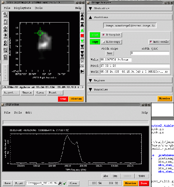
Imaging is enabled through the imager tool in DISH. It can also be executed as a script from the command line. The following is an example with comments; this assumes that the MeasurementSet has been 'patched' as shown in Section 3.

include 'imager.g'		#load the imager tool
#
#define the data to be used
thems:='/home/charybdis2/jmcmulli/jcmtdata/obs_das_0064ms'	
im:=imager(thems);		#create an imager tool

#set which data will be used; in this case each pointing is represented
#as a separate field. For this 2048 channel data, we select 500 channels
#of data from 850 to 1350 (850+500)
im.setdata(fieldid=[1:1593],spwid=1,nchan=500,start=850,step=1);

im.setoptions(gridfunction='SF')#set the gridding function to be SF
im.weight('natural');		#use natural weighting of the data

#the following defines the phase center or center of the mapped field
#this isn't really necessary for single dish data but is a required
#argument.
row:=800;
ptab:=table(spaste(thems,'/POINTING'));
direcs:=ptab.getcol('DIRECTION');
thedir:=direcs[,1,row];
global mydir:=dm.direction('J2000',spaste(thedir[1],'rad'),
       spaste(thedir[2],'rad'));

#set the image characteristics. In this case we construct a 40x40 map
#using 0.79' x 0.79' pixels. We construct a data cube with 50 planes
#which represent 10 channel averages from channel 850 to channel 1350.
im.setimage(nx=40,ny=40,cellx='0.79arcmin',celly='0.79arcmin',stokes='I',
       doshift=T,spwid=1,mode='channel',nchan=50,start=850,step=10,
       phasecenter=mydir);

#make the data cube/image. It is saved on disk as 'scanimage'
im.makeimage(image='scanimage',type='singledish');

#now view it
myimage:=image('scanimage');	#make an image tool in AIPS++ based on scanimage
myimage.view();			#calls up the viewer for seeing the image

**Figure 7.1:** Viewer display of 4 channels of the data cube. Multiple planes can be viewed by selecting the "Canvas Manager" option from the "File" menu. Also see the Getting Results chapter 3.11.
$\begin{figure} \begin{flushleft} \centering\leavevmode \vbox to6.5in{\rule{0pt... ...ffset=-50 hoffset=-220 vscale=70 hscale=70 angle=0} \end{flushleft}\end{figure}$

**Figure 7.2:** Viewer display of an image utilizing the Image Analysis Tool. Selecting the Positions Tool, choosing a position on the data cube (marked by the cross hairs), and selecting the "Auto-plot" feature allows the user to examine the gridded spectra of the data cube interactively. As each position is selected, the spectrum for that position is displayed in the lower plot.
$\begin{figure} \begin{flushleft} \centering\leavevmode \vbox to6.5in{\rule{0pt... ...ffset=-50 hoffset=-220 vscale=70 hscale=70 angle=0} \end{flushleft}\end{figure}$

7.6 To Do List for JCMT/DISH

Enable filler merge capability for multi-spectral window data
Enhance gsd->MS filler so patch script isn't needed
Enable DSB scale for plotter
Develop Frequency Switch Calibration procedure for JCMT data
Refine JCMT imaging to support standard baseline removal
Develop a Grid Spectra map utility
Enable multi-panel image display - Done.

Next: 8. Arecibo Observatory Spectral Line Reduction with DISH Up: Volume 3 - Telescope Specific Processing Previous: 6. Parkes Multibeam Reduction Contents