Version 1.9 Build 1488

News	FAQ
Search	Home

Next: 2. Processing Tabular Information Up: Volume 1 - Basic Tools Previous: Contents

Subsections

1. Plotting

Jim Braatz

1.1 Summary

This chapter provides an overview of the PGplotter tool, primarily by providing several straightforward examples which can be used to learn the basic line plotting capabilities. An example of drawing a simple raster plot is also shown, although images and arrays are better displayed in using the Viewer tool.

The aim of this document is to get users started with simple plotting. The User Reference Manual is the primary source of information about tools, and it includes comprehensive details on the PGplotter and the PGplotwidget. The Glish User Manual contains details on the native PGPLOT bindings in Glish, which implement all of the basic functions available in the PGPLOT code library.

The plotting hierarchy is that the PGplotter tool provides a standalone plotting canvas. It is built with the PGplotwidget tool, which must be embedded in some parent frame (provided in this case by the PGplotter). In turn, the PGplotwidget tool is implemented via the native Glish PGPLOT function calls.

Thus, a PGplotwidget tool has access to all of the native Glish PGPLOT functions. In turn, the higher-level PGplotter tool has access to all functions that its PGplotwidget tool has.

When using a PGplotter or PGplotwidget tool, to access the native Glish PGPLOT routines, it is only required that the '->' be replaced by '.', as shown in the examples which follow.

1.2 Creating a PGplotter `tool`

A PGplotter tool is created from the Glish prompt as follows:

include 'pgplotter.g'
pg:=pgplotter()

The specific PGplotter tool, pg, is now ready to accept plotting instructions. The following complete example shows how to make a simple line plot:

include 'pgplotter.g'
#
x := 1:100
y := sin(x/5)
pg:=pgplotter()
pg.plotxy1(x,y,'X','Y','Sample')
#
y := cos(x/3)
pg.plotxy1(x,y)              # Adds to plot with new colour

1.3 Interacting with the PGplotter

The menu bar on the PGplotter window created by the above example includes the File, Tools, Edit, and Help items.

Under the File item are the selections:

Save - allows you to save the plot either as a series of PGPLOT commands (these are stored in an AIPS++ table whose name is written to the logger).
Open - allows you to recreate a plot previously saved as PGPLOT commands with the Save selection. When Open is selected, a file browser will appear. Simply select the desired plot file from the file browser and click Send and Dismiss.
Print - activates the standard AIPS++ printer GUI. It first saves the file as a postscript file which you can then spool to a printer or preview with ghostview.
If you expect to print only a single page reflecting the current display, it is recommended that you press Clear on the PGplotter, issue the plot commands, and then send the plot to the printer. Otherwise, all plot commands stored in the buffer will be printed, possibly resulting in multiple pages of output.

Under the Tools item are the selections:

Zoom - Selecting zoom will pop up a new window which gives a Reset Full View button. Press this button to unzoom the plot to its original scale. To zoom the plot, drag out a box with the left mouse button. When the plot is zoomed as required, the zoom tool can be dismissed with the button on the zoom popup window.
Colormap - This selection allows you to modify a color table which has previously been defined by a call to the PGplotter function ctab (a native PGPLOT command). If you have not called ctab in your plot, this selection has no effect.
Dismiss - dismisses the GUI (but does not destroy it). The GUI can be recovered with the PGplotter.gui function.
Done - destroys the GUI and the PGplotter tool.

Under the Edit item are the selections:

Edit - This allows for interactive modification of the displayed plot. Selecting this will create a new GUI for editing the plot commands. The plot created by the above example is drawn with a series of 11 commands which are shown under the Drawlist column. To change the color of the line plot from red to green, for example, find the sci entry closest to the bottom of the drawlist. Select it with the left mouse button and change the ci entry from 2 to 3, then hit return and the plot will be updated. A clipboard is available to simplify any rearrangement or additions to the drawlist commands. To add new commands, the Add to Drawlist and Add to Clipboard options can be used. Simply select the command to be added from the list given and press the appropriate button. The new commands can then be seen at the bottom of the Drawlist or Clipboard list.

Under the Help menubar item are the standard AIPS++ help items, which can be used to point your web browser to appropriate help pages, report defects, and ask questions of the AIPS++ staff.

A one line message area appears just below the menu bar. Instructions for using various PGplotter tools (e.g. zoom) may appear here. Below that is the canvas for the plots.

At the bottom are buttons Save, Print, Clear, Dismiss and Done. The first and last two are short-cuts for the same operations under the menubar item File. The Clear button clears the display and empties the display list. With the Print button, you can type in the name of the file in the widget next to that button.

The PGplotter commands are most easily learned from examples. The following examples show some common plot types. For a comprehensive list of the PGplotter capabilities, see the User Reference Manual and the Glish User Manual.

1.4 Example: Reading Data from an ASCII Table and Making Plots

Suppose you have a file named SampleData.txt which contains the following data:

0.1  0.248   1.355
0.2  0.596   1.306
0.3  0.634   1.569
0.4  0.877   1.312
0.5  0.874   0.871
0.6  1.182   0.550
0.7  1.088   0.390
0.8  1.169   0.261
0.9  1.157   0.086
1.0  1.075   0.171
1.1  0.935   0.250
1.2  0.798   0.411
1.3  0.805   0.449
1.4  0.504   0.530
1.5  0.307   0.552
1.6 -0.035   1.004
1.7 -0.172   1.317
1.8 -0.232   1.648
1.9 -0.488   1.567
2.0 -0.440   1.291

Then the data can be read and plotted using the following script:

include 'table.g'
include 'pgplotter.g'
#
t := tablefromascii('sample.tbl','SampleData.txt',,T) 
t.colnames() 
#<< Column1 Column2 Column3
x  := t.getcol('Column1')
y1 := t.getcol('Column2')
y2 := t.getcol('Column3')
pg := pgplotter()
pg.plotxy1(x,y1)
pg.plotxy1(x,y2)
#
t.done()                     # Destroy tools when finished
pg.done()

The tablefromascii command (actually a constructor that constructs a Table tool called t) serves to convert the ASCII data into an AIPS++ table, which is written to disk under the name sample.tbl. The disk table can subsequently be reaccessed by connecting it to a Table tool via the constructor t := table('sample').

The next Glish statement in the example is useful during interactive sessions to list the names of the columns in the table. In this case, table t has columns named Column1, Column2, and Column 3 (the output is not shown in the example script), which are the default names given by tablefromascii when no header information is provided with the ASCII table.

The first column of the ASCII file is interpreted as the abcissa (and stored in the Glish variable x) and the numbers in the next two columns are plotted against it.

Both columns from the ASCII table are plotted on a single set of X-Y axes. The function plotxy1 can be called repeatedly to add new lines on top of the existing plot, and the scaling of the axes will be adjusted accordingly.

To plot data on the same plot but using an alternate scaling on the X-Y axes, the function plotxy2 can be used. For example, the following lines can be appended to the example to plot new data without altering the original X- and Y-scales.

xnew := 1000:2000
ynew := 100*sin((xnew-1000)/100)
pg.plotxy2(xnew,ynew)

$\begin{figure} \begin{center} \epsfig{file=cookbook.dir/plotfig1.ps,width=6.0in}\end{center}\end{figure}$

Several high level PGplotter calls, including plotxy, plotxy1, plotxy2, timey, and timey2 are intended to provide a way to take a quick look at a user's data. The functions plotxy1 and plotxy2 are intended to be used together and may not mix smoothly with plotxy or primitive PGPLOT calls in all cases. Similarly, timey and timey2 are meant to work together. When a sophisticated plot is required, it may be necessary to stick to the primitive function calls.

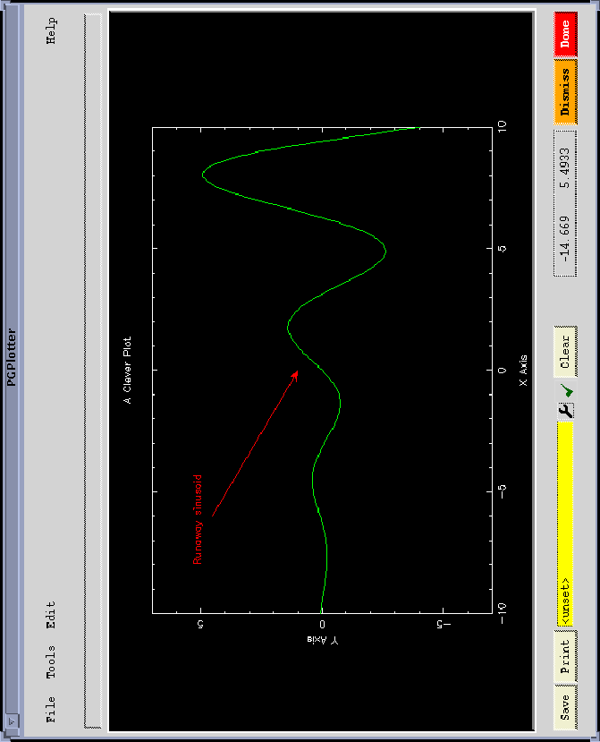
1.5 Example: Using the PGPLOT primitives

Chapter 12 of the Glish User Manual describes using direct PGPLOT bindings with Glish. A PGplotter tool is not required to use those direct bindings. However, PGplotter tools do support those methods. The only difference being that events described in the Reference Manual are replaced by functions when using the PGplotter. In practice this amounts to the '->' being replaced by '.'. For example, to set the color index use pg.sci(3) rather than pg->sci(3). The following example shows a simple plot drawn with the primitive PGPLOT commands.

include 'pgplotter.g'
#
tmp := -100:100
x:=tmp/10
y:=sin(x)*exp(x/5)
#
pg:=pgplotter()
pg.env(-10,10,-7,7,1,0)
pg.lab('X Axis','Y Axis','A Clever Plot')
pg.sci(3)
pg.line(x,y)
pg.sci(2)
pg.ptxt(-8,5,0,0,'Runaway sinusoid')
pg.arro(-6,4.5,0,1)

Consult the Glish User Manual for the comprehensive list of PGPLOT routines available.

1.6 Example: Plotting to Several Panels in a PGplotter Window

The following example shows how several plots can be drawn to individual panels on a single page. It also illustrates a simple method of plotting an image (represented as a simple Glish array) to the PGplotter window.

#
# Create some data to plot:
#
x1 := 1:100; y1 := (x1/10)^2
x2 := 1:50; y2 := log(x2)
x3 := -1000:1000
y3 := sin(x3/100)*cos(x3/100)
im := array(0,100,100)
for (i in 1:100) 
 for (j in 1:100)
  { 
  im[i,j] := i/50+sin(j/10)+random(0,10)/10
  }
#
# and plot the 4-panels:
#
include 'pgplotter.g'
pg := pgplotter()
pg.subp(2,2)
pg.env(min(x1),max(x1),min(y1),max(y1),1,0)
pg.line(x1,y1)
pg.env(min(x2),max(x2),min(y2),max(y2),0,0)
pg.line(x2,y2)
pg.env(min(x3),max(x3),min(y3),max(y3),0,0)
pg.line(x3,y3)
pg.env(1,100,1,100,1,0)
pg.gray(im,-1,4,[0,1,0,0,0,1])

Next: 2. Processing Tabular Information Up: Volume 1 - Basic Tools Previous: Contents Contents