Getting Started

Documentation

Glish

Learn More

Programming

Contact Us

Version 1.9 Build 1556

News	FAQ
Search	Home

Subsections

• Overview of commutation properties
• Overview of Jones matrix forms
• Allowable changes of order
• VisJones and SkyJones
  • Tied Array

THE ORDER OF JONES MATRICES

The Jones matrices in equation 3 generally do not commute, so their order is important. In principle, the matrices must be placed in the `physical' order, i.e. the order of the signal propagation path. But in the equations that are enshrined in existing reduction packages, this is often not the case. This begs the question why these `wrong' equations seem to produce so many good (even spectacular) results. The question is especially important since a different order often results in considerable gains in computational efficiency.

The answer is that, for existing (arrays of) circularly symmetric parabolic feeds, many Jones matrices can be approximated by matrices that do commute with at least some of the others.

Overview of commutation properties

We will analyse this in terms of those special matrices (see Appendix for their definition), whose commutation properties are:

• Unit matrices $\cal {U}$ commute with all matrices.

• Multiplication matrices $\sf Mult$(a), i.e. diagonal matrices with equal elements a, are equivalent to a multiplicative factor. Therefore, they commute with all matrices.

• Diagonal matrices $\sf Diag$(a, b) with unequal elements a, b commute with each other.

• Pure rotation matrices $\sf Rot$($\alpha$) commute with each other.

• Pseudo rotation matrices $\sf Rot$($\alpha$,$\beta$) do not commute wit each other or with pure rotation matrices $\sf Rot$($\alpha$). Moreover, there should only be one pseudo rotation matrix in the chain, and it should be to the left of (i.e. after) all other rotation matrices: $\sf Rot$($\alpha$,$\beta$)$\sf Rot$($\gamma$) = $\sf Rot$($\alpha$ + $\gamma$,$\beta$ + $\gamma$) $\neq$ $\sf Rot$($\gamma$)$\sf Rot$($\alpha$,$\beta$).

• Ellipticity matrices $\sf Ell$($\alpha$,$\beta$) do not commute with each other , except when $\beta$ = - $\alpha$. Moreover: $\sf Ell$($\alpha$,$\beta$)$\sf Ell$($\gamma$, - $\gamma$) = $\sf Ell$($\alpha$ + $\gamma$,$\beta$ - $\gamma$) $\neq$ $\sf Ell$($\gamma$, - $\gamma$)$\sf Ell$($\alpha$,$\beta$).

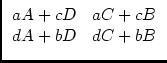
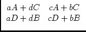
In order to study the general implications of changing the order of multiplication, we take the two products m.M and M.m of two general matrices (whose elements may be complex):

$$\left(\vphantom{\begin{array}{cc}a & c\\ d & b \end{array}}\right. \begin{array}{cc}a & c\\ d & b \end{array} \left.\vphantom{\begin{array}{cc}a & c\\ d & b \end{array}}\right) \left(\vphantom{\begin{array}{cc}A & C\\ D & B \end{array}}\right. \begin{array}{cc}A & C\\ D & B \end{array} \left.\vphantom{\begin{array}{cc}A & C\\ D & B \end{array}}\right) \left(\vphantom{\begin{array}{cc}aA+cD & aC+cB\\ dA+bD & dC+bB \end{array}}\right. \begin{array}{cc}aA+cD & aC+cB\\ dA+bD & dC+bB \end{array} \left.\vphantom{\begin{array}{cc}aA+cD & aC+cB\\ dA+bD & dC+bB \end{array}}\right)$$ =

$$\left(\vphantom{\begin{array}{cc}A & C\\ D & B \end{array}}\right. \begin{array}{cc}A & C\\ D & B \end{array} \left.\vphantom{\begin{array}{cc}A & C\\ D & B \end{array}}\right) \left(\vphantom{\begin{array}{cc}a & c\\ d & b \end{array}}\right. \begin{array}{cc}a & c\\ d & b \end{array} \left.\vphantom{\begin{array}{cc}a & c\\ d & b \end{array}}\right) \left(\vphantom{\begin{array}{cc}aA+dC & cA+bC\\ aD+dB & cD+bB \end{array}}\right. \begin{array}{cc}aA+dC & cA+bC\\ aD+dB & cD+bB \end{array} \left.\vphantom{\begin{array}{cc}aA+dC & cA+bC\\ aD+dB & cD+bB \end{array}}\right)$$ = (44)

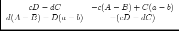
The difference (i.e. commutation error) between the two matrix products can be expressed as a matrix $\Delta$:

$$\Delta \left(\vphantom{\begin{array}{cc}cD-dC & -c(A-B)+C(a-b)\\ d(A-B)-D(a-b) & -(cD-dC) \end{array}}\right. \begin{array}{cc}cD-dC & -c(A-B)+C(a-b)\\ d(A-B)-D(a-b) & -(cD-dC) \end{array} \left.\vphantom{\begin{array}{cc}cD-dC & -c(A-B)+C(a-b)\\ d(A-B)-D(a-b) & -(cD-dC) \end{array}}\right)$$ (45)

Thus, by taking the wrong matrix order, one makes the following fractional errors of the following order in the result:  
- in the diagonal elements: of the order of c/a, i.e. the ratio of non-diagonal and diagonal elements of the original matrices (which is often small).  
- in the off-diagonal elements: in the order of (a - b)/a, i.e. they will be smaller as the diagonal elements of the original matrices are more equal.

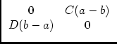
If one of the two matrices is diagonal, e.g. c  =  d  =  0 then this reduces to:

$$\left(\vphantom{\begin{array}{cc}0 & C(a-b)\\ D(b-a) & 0 \end{array}}\right. \begin{array}{cc}0 & C(a-b)\\ D(b-a) & 0 \end{array} \left.\vphantom{\begin{array}{cc}0 & C(a-b)\\ D(b-a) & 0 \end{array}}\right)$$ (46)

The (not very surprising) conclusion is that the error caused by taking the wrong matrix order is smaller when one of the matrices is diagonal, and the values of its diagonal elements are almsot equal.

Overview of Jones matrix forms

It is sufficient to discuss the commutation properties of the feed-based Jones matrices because, if A_{$\sf i$} commutes with B_{$\sf i$} and A_{$\sf j$} with B_{$\sf j$}, then (A_{$\sf i$} $\otimes$ A_{$\sf j$} ^* ) commutes with (B_{$\sf i$} $\otimes$ B_{$\sf j$} ^* ):

$$\sf J_{{\sf i}}^{} \otimes \sf J_{{\sf j}}^{\ast} \sf i \sf i \sf i \otimes \sf j \sf j \sf j \sf i \otimes \sf j \sf i \otimes \sf j \sf i \otimes \sf j$$ (47)

Inspecting the various Jones matrices separately:

  

 
$\sf F^{+}_{{\sf i}}$
= pure rotation              
$\sf Rot$($\chi_{{\sf i}}$)  

 
$\sf F^{\odot}_{{\sf i}}$
= diagonal matrix              
$\sf Diag$(expi$\chi_{{\sf i}}$, exp-i$\chi_{{\sf i}}$)  

 
$\sf T^{+}_{{\sf i}}$,$\sf T^{\odot}_{{\sf i}}$
= multiplication              
$\sf Mult$($\sf t_{{\sf i}}^{}$)  

 
$\sf K_{{\sf i}}^{}$
= multiplication             
$\sf Mult$(expi$\vec{\rho}\,$.$\vec{r}_{{\sf i}}$)                if 
$\vec{r}_{{\sf i}{\sf a}}$
= $\vec{r}_{{\sf i}{\sf b}}$
(virtually always the case)  

 
$\sf P^{+}_{{\sf i}}$
= pure rotation              
$\sf Rot$($\gamma_{{\sf x}{\sf a}}$)    if 
$\gamma_{{\sf x}{\sf a}}$
= $\gamma_{{\sf y}{\sf b}}$
 

 
$\sf P^{\odot}_{{\sf i}}$
= diagonal matrix              
$\sf Diag$(expi$\gamma_{{\sf x}{\sf a}}$, exp-i$\gamma_{{\sf x}{\sf a}}$)    if 
$\gamma_{{\sf x}{\sf a}}$
= $\gamma_{{\sf y}{\sf b}}$
 

 
$\sf P^{+}_{{\sf i}}$
= pseudo-rotation              
$\sf Rot$($\gamma_{{\sf x}{\sf a}}$,$\gamma_{{\sf y}{\sf b}}$)    if 
$\gamma_{{\sf x}{\sf a}}$
$\neq$
$\gamma_{{\sf y}{\sf b}}$
 

 
$\sf P^{\odot}_{{\sf i}}$
= A general matrix    if 
$\gamma_{{\sf x}{\sf a}}$
$\neq$
$\gamma_{{\sf y}{\sf b}}$
 

 
$\sf E^{+}_{{\sf i}}$,$\sf E^{\odot}_{{\sf i}}$
= diagonal matrix              
$\sf Diag$($\sf e_{{\sf i}{\sf a}{\sf a}}^{}$,$\sf e_{{\sf i}{\sf b}{\sf b}}^{}$)                 if  no cross-leakage              (
$\sf e_{{\sf i}{\sf a}{\sf b}}^{}$
= $\sf e_{{\sf i}{\sf b}{\sf a}}^{}$
= 0)  

		 = multiplication             
$\sf Mult$($\sf e_{{\sf i}}^{}$)                if also 
$\sf e_{{\sf i}{\sf a}{\sf a}}^{}$
= $\sf e_{{\sf i}{\sf b}{\sf b}}^{}$
for all 
$\vec{\rho}\,$
 

 
$\sf D^{+}_{{\sf i}}$,$\sf D^{\odot}_{{\sf i}}$
$\approx$
unit matrix $\cal {U}$
   if small leakage, i.e.              (
$\sf d_{{\sf i}{\sf a}{\sf b}}^{}$
$\approx$
$\sf d_{{\sf i}{\sf b}{\sf a}}^{}$
$\approx$
0)

 

 
$\sf D^{+}_{{\sf i}}$
=              
$\sf Ell$($\theta_{{\sf i}{\sf a}}$,$\theta_{{\sf i}{\sf b}}$)             
$\sf Rot$($\phi_{{\sf i}{\sf a}}$,$\phi_{{\sf i}{\sf b}}$)   

		 $\approx$

$\sf Ell$($\theta_{{\sf i}{\sf a}}$, - $\theta_{{\sf i}{\sf a}}$)             
$\sf Rot$($\phi_{{\sf i}{\sf a}}$)                if 
$\theta_{{\sf i}{\sf b}}$
= - $\theta_{{\sf i}{\sf a}}$
and 
$\phi_{{\sf i}{\sf b}}$
= $\phi_{{\sf i}{\sf a}}$
 

 
$\sf D^{\odot}_{{\sf i}}$
=              (
$\cal {H}$ $\sf Ell$($\theta_{{\sf i}{\sf a}}$,$\theta_{{\sf i}{\sf b}}$) $\cal {H}$-1)             (
$\cal {H}$ $\sf Rot$($\phi_{{\sf i}{\sf a}}$,$\phi_{{\sf i}{\sf b}}$) $\cal {H}$-1)  

		 $\approx$

$\sf Rot$($\theta_{{\sf i}{\sf a}}$)             
$\sf Diag$(expi$\phi_{{\sf i}{\sf a}}$, exp-i$\phi_{{\sf i}{\sf a}}$)                 if 
$\theta_{{\sf i}{\sf b}}$
= - $\theta_{{\sf i}{\sf a}}$
and 
$\phi_{{\sf i}{\sf b}}$
= $\phi_{{\sf i}{\sf a}}$
 

 
[$\sf Y_{{\sf i}}^{}$] = anti-diagonal matrix: a problem, if present....   

 
[$\sf H_{{\sf i}}^{}$] = effectively hidden if present,                           see equation 24  

 
$\sf G_{{\sf i}}^{}$
= diagonal matrix             
$\sf Diag$($\sf g_{{\sf i}{\sf p}{\sf p}}^{}$,$\sf g_{{\sf i}{\sf q}{\sf q}}^{}$)    if no cross-talk 

Problems are caused predominantly by matrices with non-zero off-diagonal elements like $\sf D_{{\sf i}}^{}$, $\sf Y_{{\sf i}}^{}$, and $\sf P_{{\sf i}}^{}$ if $\gamma_{{\sf x}{\sf a}}$ $\neq$ $\gamma_{{\sf y}{\sf b}}$. Of these, only $\sf D_{{\sf i}}^{}$ is present in all telescopes. $\sf P_{{\sf i}}^{}$ will be a problem for SKAI, bacause $\gamma_{{\sf x}{\sf a}}$ $\neq$ $\gamma_{{\sf y}{\sf b}}$.

Allowable changes of order

The following changes in the order of Jones matrices is allowed, but only under the indicated conditions. NB: Some Jones matrices will commute if it can be assumed that the observed source is compact, dominating, unpolarised and near the centre of the field. This is often the case.

• If the Faraday angle does not vary over the primary beam, $\sf F_{{\sf i}}^{}$ might be applied in the uv-plane. $\sf F_{{\sf i}}^{}$ will in general commute with $\sf P_{{\sf i}}^{}$ except when $\sf P_{{\sf i}}^{}$ is a pseudo-rotation ( $\gamma_{{\sf x}{\sf a}}$ $\neq$ $\gamma_{{\sf y}{\sf b}}$). $\sf F^{\odot}_{{\sf i}}$ is diagonal, and will commute with $\sf E_{{\sf i}}^{}$ if it is diagonal. But $\sf F^{+}_{{\sf i}}$ will only commute with $\sf E_{{\sf i}}^{}$ if the latter is a multiplication. If there is appreciable cross-leakage, $\sf F_{{\sf i}}^{}$ should stay to the right of $\sf D_{{\sf i}}^{}$, which means that in that case $\sf F^{\odot}_{{\sf i}}$ cannot be lumped with $\sf G_{{\sf i}}^{}$ as is often done.

• $\sf T_{{\sf i}}^{}$ is a multiplication, which commutes with everything. If it does not vary over the primary beam, it can be lumped with $\sf G_{{\sf i}}^{}$.

• If the two receptors of a feed are located at the same position (which is virtually always the case), the FT kernel matrix $\sf K_{{\sf i}}^{}$($\vec{\rho}\,$.$\vec{r}_{{\sf i}}$) reduces to a multiplication $\sf k_{{\sf i}}^{}$($\vec{\rho}\,$.$\vec{r}_{{\sf i}}$). This means that the FT can be performed at any desired place in the chain, even to the right of the Stokes matrix. NB: If $\vec{r}_{{\sf i}{\sf a}}$ $\neq$ $\vec{r}_{{\sf i}{\sf b}}$, it would not be trivial to figure out what the correct position of $\sf K_{{\sf i}}^{}$ should be.

• If the map centre $\vec{\rho}_{mc}$ is different from the fringe tracking centre $\vec{\rho}_{ftc}$, the FT kernel may be split into a product: $\sf K_{{\sf i}}^{}$($\vec{\rho}\,$.$\vec{r}_{{\sf i}}$)  =  $\sf K^{0}_{{\sf i}}$($\vec{\rho}_{mc}$.$\vec{r}_{{\sf i}}$) $\sf K^{'}_{{\sf i}}$(($\vec{\rho}\,$ - $\vec{\rho}_{mc}$).$\vec{r}_{{\sf i}}$). Since $\vec{\rho}_{mc}$ does not depend on source position, $\sf K^{0}_{{\sf i}}$($\vec{\rho}_{mc}$.$\vec{r}\,$) may be moved to the leftmost part of the chain, i.e. to the uv-plane part.

• If $\sf E_{{\sf i}}^{}$($\vec{\rho}\,$) = $\sf E_{{\sf j}}^{}$($\vec{\rho}\,$) = $\sf Mult$($\sf e$($\vec{\rho}\,$)), i.e. if all voltage patterns are identical, then $\sf E_{{\sf i}{\sf j}}^{}$ = ($\sf E_{{\sf i}}^{}$ $\otimes$ $\sf E_{{\sf j}}^{\ast}$) commutes with the Stokes matrix $\sf S$ and may be applied directly to the Stokes vector $\vec{I}\,$ in the image plane. This condition is more likely to occur near the beam centre. NB: Because $\sf E_{{\sf i}{\sf j}}^{}$ does definitely not commute with $\sf S$ if $\sf e_{{\sf i}{\sf a}{\sf a}}^{}$ $\neq$ $\sf e_{{\sf i}{\sf b}{\sf b}}^{}$, the justification for the practice of applying off-axis instrumental polarisation to $\vec{I}\,$ seems a little doubtful.

• $\sf P_{{\sf i}}^{}$ may be moved to the left of $\sf E_{{\sf i}}^{}$ if they are both diagonal matrices, or if $\sf E_{{\sf i}}^{}$ is a multiplication. Since $\sf P^{\odot}_{{\sf i}}$ is diagonal and $\sf P^{+}_{{\sf i}}$ is not (except for equatorial mounts), this appears to be an argument in favour of the use of circular polarisation coordinates. If $\sf E_{{\sf i}}^{}$ is diagonal and almost a multiplication (i.e. $\sf e_{{\sf i}{\sf a}{\sf a}}^{}$ $\approx$ $\sf e_{{\sf i}{\sf b}{\sf b}}^{}$), $\sf P^{+}_{{\sf i}}$ may be moved to the left of $\sf E_{{\sf i}}^{}$ at the cost of a small error of the order ($\sf e_{{\sf i}{\sf a}{\sf a}}^{}$ - $\sf e_{{\sf i}{\sf b}{\sf b}}^{}$)/$\sf e_{{\sf i}{\sf a}{\sf a}}^{}$ (see equation 47).

• If $\sf P_{{\sf i}}^{}$ and $\sf E_{{\sf i}}^{}$ do not commute at all, one can still move $\sf P_{{\sf i}}^{}$ to the left of $\sf E_{{\sf i}}^{}$ by using $\sf E_{{\sf i}}^{}$ $\sf P_{{\sf i}}^{}$  =  $\sf P_{{\sf i}}^{}$ ($\sf P_{{\sf i}}^{-1}$ $\sf E_{{\sf i}}^{}$ $\sf P_{{\sf i}}^{}$)  =  $\sf P_{{\sf i}}^{}$ $\sf E_{{\sf i}}^{''}$
  Since this re-introduces time-dependent off-diagonal elements into $\sf E_{{\sf i}}^{''}$, it is not clear how useful this is.

VisJones and SkyJones

The Jones matrices may split up in two groups: $\sf J_{{\sf i}}^{}$  =  $\sf J^{vis}_{{\sf i}}$ $\sf J^{sky}_{{\sf i}}$. In these terms, the full M.E. (ignoring normalisation factors, see equ 6) becomes:

$$\vec{V}_{{\sf i}{\sf j}} \int \sf t \int \sf f \sf J^{vis}_{{\sf i}} \otimes \sf J^{vis}_{{\sf j}}^{\ast} \sum_{{k}}^{} \int \sf l \sf m \sf J^{sky}_{{\sf i}} \otimes \sf J^{sky}_{{\sf j}}^{\ast} \sf S \vec{I}_{k}$$ (48)

We now see the reason for placing the integration over $\sf f$ and $\sf t$ to the left of the sum over k sources. Since it is computationally advantageous to minimise the number of Jones matrices that operate in the image plane, it must be investigated whether Jones matrices that do not depend on the source position can be moved to the left in the chain, using the rules in section 6.3 above. Depending on the chosen coordinate system, (and always keeping in mind the conditions for re-ordering Jones matrices), the following split appears to be the maximum obtainable:

$$\sf J^{vis}_{{\sf i}} \sf K^{0}_{{\sf i}} \sf G_{{\sf i}}^{} \sf T_{{\sf i}}^{} \sf D^{+}_{{\sf i}} \sf P^{+}_{{\sf i}} \sf F^{+}_{{\sf i}} \sf S \sf S^{+}_{}$$ = (49)

$$\sf K^{0}_{{\sf i}} \sf G_{{\sf i}}^{} \sf T_{{\sf i}}^{} \sf F^{\odot}_{{\sf i}} \sf D^{\odot}_{{\sf i}} \sf P^{\odot}_{{\sf i}} \sf S \sf S^{\odot}_{}$$ = (50)

$$\sf J^{sky}_{{\sf i}} \sf E_{{\sf i}}^{} \sf K^{'}_{{\sf i}}$$ = (51)

This is what is done implicitly in some existing reduction packages.

Tied Array

For a tied array (ignoring integration and weight factors for the moment), equation 5 becomes:

$$\vec{V}_{{\sf i}{\sf j}} \sf Q_{{\sf i}}^{} \otimes \sf Q_{{\sf j}}^{\ast} \sum_{{n}}^{} \sum_{{m}}^{} \sf J^{vis}_{{\sf i}n} \otimes \sf J^{vis}_{{\sf j}m}^{\ast} \sum_{{k}}^{} \sf J^{sky}_{{\sf i}nk} \otimes \sf J^{sky}_{{\sf j}mk}^{\ast} \sf S \vec{I}_{k}$$ (52)

Under extremely favourable conditions, i.e. if:  
- individual feed beams per tied array are identical.  
- Faraday rotation is the same for an entire tied array  
- All receptors of a tied array have the same orientation.  
- receptor cross-leakages are small.  
- tied array feed signals are corrected before adding.  
- there are no delay errors.  
then equation 53 can be reduced to:

$$\vec{V}_{{\sf i}{\sf j}} \sf Q_{{\sf i}}^{} \otimes \sf Q_{{\sf j}}^{\ast} \sf P_{{\sf i}}^{} \otimes \sf P_{{\sf j}}^{\ast} \sf F_{{\sf i}}^{} \otimes \sf F_{{\sf j}}^{\ast} \sum_{{k}}^{} \sf E_{{\sf i}k}^{} \otimes \sf E_{{\sf j}k}^{\ast} \sum_{{n}}^{} \sum_{{m}}^{} \sf K_{{\sf i}nk}^{} \otimes \sf K_{{\sf j}mk}^{\ast} \sf S \vec{I}_{k}$$ (53)